Journal of Environmental Protection
Vol. 4 No. 7A (2013) , Article ID: 34848 , 9 pages DOI:10.4236/jep.2013.47A016
Effect of the Application of Produced Water on the Growth, the Concentration of Minerals and Toxic Compounds in Tomato under Greenhouse
![]()
1Departamento de Horticultura, Universidad Autónoma Agraria Antonio Narro, Saltillo, México; 2Departamento de Fitomejormamiento, Universidad Autónoma Agraria Antonio Narro, Saltillo, México.
Email: josefernandomartelvalles@yahoo.com.mx, *abenmen@uaaan.mx, luisalonso_va@hotmail.com, juma841025@hotmail.com, nruiz@uaaan.mx
Copyright © 2013 José Fernando Martel-Valles et al. This is an open access article distributed under the Creative Commons Attribution License, which permits unrestricted use, distribution, and reproduction in any medium, provided the original work is properly cited.
Received June 13th, 2013; revised July 10th, 2013; accepted July 15th, 2013
Keywords: Congenital Water; Salt Content; THP; NOM-143-SEMARNAT-2003
ABSTRACT
During the production of petroleum and gas a by-product, known as congenital water, is obtained, which varies in composition depending on the geological formation from which it is extracted. In the industrial process its composition is modified and then it is known as “produced water”. These waters can contain high concentrations of mineral salts that can potentially be used for crop fertilization. The aim of this study was to evaluate the effects of the application of produced water on the mineral contents of the plants and levels of BTEX and TPH in the fruits of greenhouse tomato cultivation. The produced waters used were derived from gas producing zone of Sabinas-Piedras Negras in northern Mexico. These waters were analyzed according to NOM-143-SEMARNAT-2003. Waters from three different stations, (Buena Suerte, Forasteros and Monclova 1), were mixed with fresh water to obtain the treatment waters used. As a control, we used a complete Steiner solution. The results showed that the produced waters modified the absorption of essential minerals in tomato plants; it was observed that the mineral concentration in plant tissues was highest in the control plants, except for Na, in which the plants irrigated with produced water had the highest concentrations. The treatments with produced waters also affected negatively the root length, leaf dry weight, stem dry weight, number of fruits per plant, and the dry weight of the fruits.
1. Introduction
Congenital water or connate water is the water trapped in the pores of sediment in the moment of their formation. This water can contain a large quantity of salts and become part of rock and minerals as water adsorbed in clays. Considering that this water does not evaporate nor circulate between different strata, it has not been considered part of the hydrological cycle [1,2]. In 2002, 12.09 × 10⁶ m3 of produced water was generated in México [3], and in 2010 there were 12.04 × 10⁶ m3, according to information provided by Petróleos Mexicanos, in the document named Reporte de Responsabilidad Social [4]. In México, NOM-143-SEMARNAT-2003 [3] has established the environmental specifications for the management of congenital water (produced water) associated with hydrocarbon exploitation. The norm establishes the acceptable limits for compounds contained in this water, as well as the forms authorized in México for the disposal of these waters. The most common technique used is to increase output of hydrocarbons by the injection of produced water into productive wells [3,5]. In respect to its physiochemical composition and volume, the produced waters show variation depending on the extraction site, and the age and the geology of the formation from which the oil and gas is produced [6-8]. Various studies have indicated a great variability in the characteristics of salinity and content of elements of the produced water, and such variability can obtain even between hydrocarbon extraction sites in relatively close proximity1. This variation occurs in the same way in the produced water derived from marine platforms [4,9]. Some sources of produced water contain high salt content, as much as five or six times as much as sea water. They also may contain concentrations of Cl− 150,000 to 180,000 mg·L−1 (sea water contains an average of 35,000 mg·L−1) and show an average electrical conductivity (EC) of 3200 dS·m−1 [10]. With these levels of salts the water is toxic for many forms of life [11,12]. For crop plants the irrigation water is considered saline when the electrical conductivity is more than 3 dS·m−1 or 2000 mg·L−1 of total dissolved solids (TDS) [8,13,14]. In addition, the produced water can contain compounds of low molecular weight, organic acids, condensers, oils and fats, aromatic hydrocarbons such as benzene, toluene, ethylbenzene, xylene, polycyclic hydrocarbons (PAH) and phenols [7]. When present in the water, these compounds contribute to the toxicity, individually and together [7,8]. It can also contain chemical additives used during the drilling and production operations [8]. The concentration of metals in the produced water depends on the specific site, the characteristics and age of the geologic formation from which the petroleum or gas is produced [7]. Normally, the waters derived from gas wells contain several times greater concentration of metals than that derived from oil wells [15].
There are industrial uses for produced water [8,16], which will not be considered here. Also, it is commonly used for injection into oil wells to increase output (fracking). Agricultural uses include irrigation of vegetable crops in soil and hydroponic trough for livestock or wildlife [7,17]. It has been shown experimentally that some types of produced water, with low salt content, are feasible for such agricultural uses [7,16]. Since in México there is not sufficient information available about the use of the produced waters, and its effects on greenhouse crops, the objective of this study was to evaluate the effect of produced water application on tomato plants under greenhouse conditions verifying growth and the contents of minerals and toxic compounds in plant tissues.
2. Materials and Methods
The experimental work was performed in the greenhouse of the Departamento Forestal at Universidad Autónoma Agraria Antonio Narro located in Buenavista, Saltillo, Coahuila, México, whose geographic coordinates are: north latitude, 25˚22′ West longitude 101˚00′, at an altitude of 1760 meters above sea level.
2.1. Produced Waters
The produced water utilized for the present study was obtained from three PEMEX gas producing wells (Buena Suerte, Monclova 1 and Forasteros) located in the municipalities of San Buenaventura, Monclova and Abasolo, located in the gas production area Sabinas-Piedras Negras of Coahuila State, México. Each of these stations gets portions of produced water from as many as 25 wells; therefore the water from each station was a mixture from different nearby wells. These stations were selected because of the high electrical conductivity values of their produced waters.
In order to characterize the produced water taken from the three stations, some samples were analyzed according to the NOM-143-SEMARNAT-2003 [3]. For comparative purposes a complete Steiner Solution [18] at 75% concentration was also analyzed under this norm. This analysis took into account the hydrocarbons (fraction light, medium and heavy), fats and oils, and also considered the concentrations of Zn+2, Pb+2, Ni+2, Cd+2, Cu+2, Hg+2, As+3, Cr+3 total nitrogen, total phosphorous, nitrogen as nitrates, nitrogen as nitrites, and the sum of nitrogenous compounds. We also assessed the pH, the biochemical demand of oxygen (BDO), solid sediments, floating matter, total solids, total dissolved solids (TDS), total suspended solids (TSS) and total volatile solids (TVS).
2.2. Formulation and Application of Treatments
In preparing the mixtures to be applied to the tomatoes we took into account the EC from each one of the produced water samples. A dilution of the produced waters was made with the available fresh water in the greenhouse, to achieve an EC value approximately equal to the fertilizer solution (Steiner), applied at each of the phenological stages. Finally, the pH of each mixture was adjusted to a value of approximately 6.0. These mixtures were then used for irrigation treatments on the plants (Table 1). As a control application (T0), only the Steiner fertilizer solution [18] was used. This solution was administered in different concentrations according to the phenological stage of the plant.
2.3. The Cultivation and Treatment Applications
The cultivation in the greenhouse was done from April 30th to August 24th, 2012. Tomato plants, hybrid saladette (Solanum lycopersicum L.) variety “El Cid,” with an undetermined growth pattern, were used. The seed plant was produced in 200 cavity polystyrene trays, using as substrate a mixture of peat moss and perlite (3:1). The
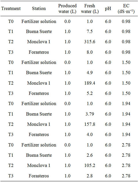
Table 1. Description of the treatments. Shows the proportion of produced water with the fresh water used in different phenological stages.
transplant was done in black polystyrene pots with a volume of 16 liters in a substrate mixture of peat moss and perlite (3:1). A system of soil-less cultivation was utilized, and an irrigation system was conducted through high flow stakes. The plants were pruned to a single stem and were cultivated by a standard method.
In order to obtain plants with homogeneous vigor and growth, they were watered only with the fertilizing solution for 23 days before initiating treatments. Application of waters was done three times per day, at 9:00, 13:00 and 18:00 hours, applying around 800 ml per plant. Produced water treatment application was done in the first and third watering, while in all cases the fertilizing solution was applied in the second watering.
2.4. Morphologic Variables Assessed
The morphologic variables determined in tomato plants were the stem diameter (SD) (mm) measured in the first internode on the stem base utilizing a digital Vernier calibrator. The height of the plant (H) (cm) was measured from the stem base to the terminal bud, and the root length (RL) (cm) was measured from the base of the stem to the central root cap. To measure these variables a measuring tape was used. Dry weight (g) of the leaves (LDW) and stem (SDW) was obtained in the flowering stage (30 days after transplanting, DAT), and in the fructification stage (108 DAT). The dry weight of leaves (LDW), stems (SDW) and fruits (FDW) was determined in separate measurements. In both stages the weight was measured after drying in the dehydrating stove at 60 degrees Celsius for three days. An analytical scale, brand OHAUS, model SCOTPROSP6000 was used. To determine the number of fruits per plant (FN), five plants per treatment during the fructification stage were chosen at random. In these plants the number of fruits was counted in every cut. The dried fruit per plant (g) (DFP) was gotten from the sum of six cuts during the harvest stage between the 78 and 108 DAT. In this case the dry weight was measured after drying in an oven at 60˚C dehydration during four days.
2.5. Mineral Contents in the Plants
In order to determine mineral content (N, P, K, Ca, Mg, Na, Fe, Cu, Zn, Mn, Mo, Ni, Cd, Pb and Cr), five plants per treatment group were chosen at random in the flowering stages (30 DAT) and fructification stage (108 DAT). In the flowering stage, root steam and leaf were collected; while in the fructification stage, root, steam, leaf and fruit samples were collected. The samples were dried in a dehydrating stove at 60˚C, pulverized and subjected to acid digestion, to be later analyzed with an atomic absorption spectrophotometer brand Varian AA, according with AOAC [19]. The phosphorus was determined by the Olsen method [19] utilizing a spectrometer UV-Vis model Helios Epsilon of wave-length 640 nm. The nitrogen was determined by using the macro Kjeldhal method in conformance with the standard techniques [19].
2.6. MFH and BTEX Content in Fruit
To verify the possible accumulation of toxic substances in the fruits produced by tomato plants treated produced water mixtures, fruits were analyzed to measure the concentration of hydrocarbons from the middle fraction (MFH) and aromatic hydrocarbons benzene, toluene, ethylbenzene and xylenes (BTEX). For MFH analysis method EPA-8015B-1996 [20] was used, while for BTEX analysis method EPA-8260C-2006 [21] was used.
2.7. Statistical Analysis
The experimental procedure was totally at random, with 26 repetitions per treatment in the case of morphology variables, but in the case of mineral analysis only five repetitions were considered. The experimental unit was a pot with a plant. For this analysis we utilized a variance analysis (ANOVA) and a measure test according to Tukey (a ≤ 0.05). For this, software SAS [22] was used.
3. Results and Discussion
3.1. Analysis of Produced Water
Results of the analysis of produced waters made according to NOM-143-SEMARNAT-2003 [3] are depicted in Table 2. In addition, we included for comparative pur-
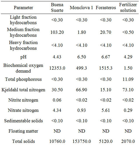
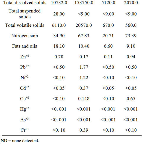
Table 2. Analysis of produced waters according to the NOM-143-SEMARNAT-2003 (SEMARNAT 2003a) referenced to the Steiner (1961) at 75%, also analyzed according to the same norms. All concentrations are expressed in mg·L−1, except for pH.
poses the fertilizer solution Steiner [18] at a 75% concentration, verified under the same official regulation. The results show that the produced water coming from either Buena Suerte or Forasteros station had high hydrocarbon content according to NOM-143-SEMARNAT- 2003 [3]. These waters could cause toxicity in soil and crops if used as irrigation water [23-25], provoking physiological problems such as germination inhibition, vegetal growth suppression or plant death [26]. None of the produced waters exceeded the permissible maximum limit of fats and oils for irrigation waters, according to NOM-001-SEMARNAT-1996 [27]. We further determined that the produced water in Buena Suerte station was out of the pH optimal range to be used as irrigation water [13,28]. It was observed that the total volatile solids (TVS), and total dissolved solids (TDS) and volatile solids (VS) of produced waters in Buena Suerte and Monclova 1 stations were above limit of NOM-001- SEMARNAT-1996 [27]. Besides, the total phosphorous in the produced waters from all stations was in no way optimal [26], nor were the nitrates and nitrites, according to the FAO [13]. On the contrary, the total nitrogen level in the water from Monclova 1 station and in the fertilizing solution was above indicated norms of NOM-001- SEMARNAT-1996 [27]. Regarding the minerals, the water from Monclova station 1 was out of permissible range for Pb according to NOM-001-SEMARNAT-1996 [27] and was over the toxic threshold according to the guide, ARPEL [12]. All the other minerals were inside the limits set by the NOM-001-SEMARNAT-1996 [27] (Table 2).
3.2. Morphological Variables Evaluated
Table 3 depicts the results of the morphological variables assessed in tomato plants during the crop development. The results are shown in flowering stage (30 DAT) and fructification stage (108 DAT). We can see that in the flowering stage the RL shows statistical differences, while the rest of the variables evaluated in this stage (H, SD, LDW and SDW) between treatments are equal. Notably, the T2 treatment corresponding to Monclova 1 station presented the highest root length, while the T1 treatment corresponding to Buena Suerte station had the lowest root length (Table 3).
In the fructification stage, it was observed that only the variables H and SD showed no statistically significant differences. As for the variables, RL, LDW, SDW, FN and DFP clear differences were observed in all cases showing that the T1 treatment was statistically the lowest. Also it was found that T0 treatment showed the highest values in LDW, SDW, FN and DFP variables (Table 3). The results obtained in this stage can be attributed to the mineral content in the tissues of plants, since T1 consis-
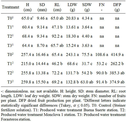
Table 3. Average values for the morphologic variables evaluated in tomato plants that were irrigated with produced water using the irrigation system. Data shows flowering1 and fruiting2 stages.
tently presented the lowest concentrations and the opposite was true for T0 (fertilizer solution Steiner), which presented the highest concentrations (Tables 4-7). Since the content of hydrocarbons was especially high in the water sample of T1, the negative response can be attributed to those hydrocarbons which are known to cause toxicity [23,24] and oxidative stress [29] in plants. Also, these results agree with Jackson and Myers [30], and although it is feasible the use of water produced in plants, those who were treated only with nutrient solution (T0) showed better results (Table 3).
3.3. Mineral Content in Plant Tissues
The results of the concentration of minerals in the root of the tomato plants both for the flowering stage and fruiting stage are showed in Table 4. Considering that the concentration of minerals by the treatments was highly variable, we were to be expected significant differences in mineral content of plant tissues. Nevertheless at the flowering stage it was observed that the concentration of N, P, K, Ca, Fe, Cu, Mn, Mo, Ni, Cd, Pb and Cr showed no statistically significant differences. At this stage only the concentration of Mg, Na and Zn were statistically different: with the plants irrigated with water corresponding to T1 Buena Suerte station with the lowest concentration of these minerals (Table 4). In the fruiting stage statisticcally significant differences in minerals N, Na, Cu, and Mn were found. For most of the minerals (P, K, Ca, Mg, Fe, Zn, Ni, Cd, Pb and Cu) again there were no significant differences. Also, it was observed that the T0 (Steiner fertilizer solution) had the highest concentration of N, Cu, Mn and Mo. On the other hand, for Na, the T0 solution showed the lowest concentration (Table 4).
Table 5 presents the results of the concentration of minerals in the stem of the tomato plants during the stages of flowering and fruiting. In the flowering stage only N, Mg, and Na, of the 15 evaluated mineral, showed statistical differences. It can be seen that the T0 presented the highest concentration of N while for Na showed the lowest concentration. It was further shown that the T1 had the highest concentration of Na and the lowest Mg concentration (Table 5). In the fruiting stage it was found that the concentrations of Fe, Mo, Ni, Cd, and Pb were statistically equal between treatments. It is also observed that for the concentration of N, P, K, Ca, Mg, Cu, Mn and Cr, T0 was the greatest, while for T1 it is the

Table 4. Concentration of minerals in the root of the tomato plants receiving produced water through the irrigation system. Data shows flowering1 and fruiting2 stages.
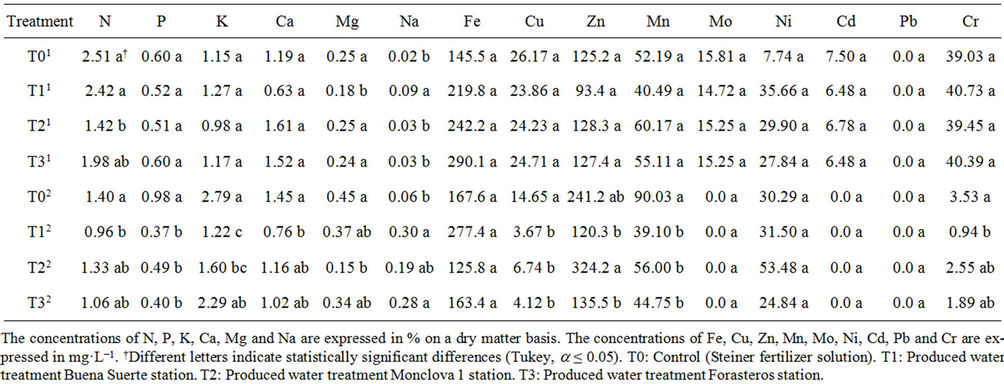
Table 5. Concentration of minerals in the stem of the tomato plants receiving produced water through the irrigation system. Data shows flowering1 and fruiting2 stages.
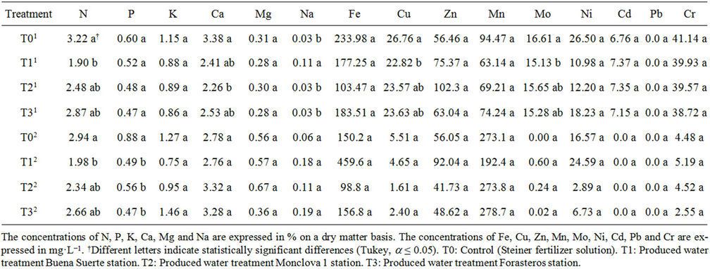
Table 6. Concentration of minerals in the leaf of the tomato plants receiving produced water through the irrigation system. Data shows flowering1 and fruiting2 stages.
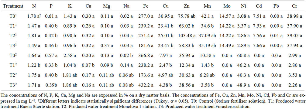
Table 7. Concentration of minerals in the fruit of the tomato plants receiving produced water through the irrigation system. Data present the results of the first1 and sixth2 picking.
inverse, since with the exception of Mg, T1 had the lowest concentration in all the above minerals (Table 5).
The concentration of minerals in the leaf of tomato plant is presented in Table 6. As in previous cases, we considered the stages of flowering and fruiting. In the flowering stage it was found that mineral N, Ca, Na, Cu and Mo showed statistically significant differences, while the rest were the same (P, K, Mg, Fe, Zn, Mn, Ni, Cd, Pb and Cr). It was observed also that for N, Ca, Cu and Mo, T0 had the highest concentration, while T1 had the highest concentration of Na (Table 6). In the case of the fruiting stage, it was found that only the concentration of N and P presented statistical differences between treatments. It was further observed that for the mineral content in both stages, T0 had the highest concentration (Table 6).
Finally, the concentrations of minerals in the fruit of tomato plants, considering the first and sixth cut, are shown in Table 6. It can be appreciated that in the first cut only the concentration of P, K, Cu, Zn and Mn showed statistical differences between treatments. For the remaining minerals (N, Ca, Mg, Na, Fe, Mo, Ni, Cd, Pb and Cr), no significant differences were obtained between treatments. It is observed that in terms of P, K, Cu and Mn, T0 was the highest concentration, while for Zn, T2 (corresponding to Monclova 1 station) was higher than the other treatments. In the sixth cut was observed that there were statistically significant differences between treatments in the concentration of N, P, K, Ca, Mg, Na, Cu and Mn. Also it is seen that in all cases consistently, with the exception of Na, the T1 had the lowest concentration. Also in terms of the concentration of Na, T1 was a higher concentration (Table 7).
It was systematically observed that minerals, except Na, when there were differences between treatments, the T0 had the highest concentrations tested (Tables 4-7). This phenomena can be explained because the T0 only applied Steiner solution, which ensured that all mineral elements required by the plant were available [18], thus facilitating their absorption by the plant. In the case of treatments with produced water, it was found that these showed great variability in their physicochemical composition and salt content [6-8] that might interfere with the absorption of different minerals by plants. Coupled with this, the presence of hydrocarbons in produced water could damage the root structure of the tomato plant due to its toxic effect [7,8], which consequently limited the absorption of the minerals needed for the plant.
In most cases where there were significant differences in the concentration of Na in different tissues, the T1 was the greatest (Tables 5-7). It is known that the Na is one of the major cytotoxic ions [31], and contributes to ion imbalances triggered in plants by excessive absorption, which generates toxicity and side effects associated with the nutritional problem of ion uptake essential for growth and development of plants [32]. So this can account for why the plants treated with T1 (treatment Buena Suerte) showed lower mineral content (Tables 4-7), which was also reflected in the morphologic variables (Table 2).
3.4. MFH and BTEX Content in Fruit
Table 8 presents the results of the analysis of the fruits of tomato plants under methods EPA-8015B-1996 [20] and EPA-8260C-2006 [21]. It was found that none of the treatments produced an accumulation of toxic compound (MFH, benzene, toluene, ethylbenzene and xylenes). There is evidence that total petroleum hydrocarbons (TPH) can cause toxicity in multiple organisms for different reasons. At the cellular level plants are capable of producing free radicals, which can damage cell structure and DNA [33], from direct contact [34], or from absorption through the stomata or roots [35]. Considering the above, the results are an indication that in this particular case possibly plants were unable to absorb any type compound MFH and BTEX (Table 8). Moreover, there was a negative effect on the root, as the treatment with Buena Suerte station water was lower than the other treatments by about 30% based on the root length (Table 3), which may be due to damage by direct contact [34]. Considering these two facts, it is possible that the roots of the tomato plants are very susceptible to petroleum compounds, so that when in contact with these, it generates a direct damage to the root which prevents proper absorption.
4. Conclusions
Produced waters use growing greenhouse tomato is feasible. However, the effectiveness of its use will depend
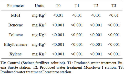
Table 8. Hydrocarbon concentration of middle fraction (MFH) and aromatic hydrocarbons in the fruits of tomato plants were produced water through the irrigation system. The results correspond to fruit samples collected from first, third and sixth picking.
on the biochemical characteristics of the waters used.
Produced water significantly affects the absorption of essential minerals by tomato plants, and can affect the growth of same. Therefore, growers should pay particular attention to the content of salts produced by the different waters if they want to use these waters for growing greenhouse vegetables.
The fruits of tomato plants showed no accumulation of toxic petroleum such as middle fraction hydrocarbons or aromatic compounds such as benzene, toluene, ethylbenzene and xylenes.
REFERENCES
- L. D. Leet and S. Judson, “Fundamentos de Geología Física,” Editorial Limusa-Wiley, México D.F., 1974.
- J. Llamas, “Hidrología General. Principios y Aplicaciones,” Editorial Universitaria del País Vasco, Bilbao, 1993.
- SEMARNAT, “Norma Oficial Mexicana NOM-143- SEMARNAT-2003, Que Establece las Especificaciones Ambientales para el Manejo de agua Congénita Asociada a Hidrocarburos,” Secretaría de Medio Ambiente Recursos Naturales y Pesca, Diario Oficial de la Federación, 2005.
- PEMEX, “Informe de Responsabilidad Social,” 2010. http://www.pemex.com/informes/pdfs/descargas/pemex_irs_completo_2011.pdf
- CNH, “Documento Técnico 1 (DT-1), Factores de Recuperación de Aceite y gas en México,” 2010. http://www.cnh.gob.mx/_docs/DOCUMENTOTECNICO1FINAL.pdf
- R. Lee, R. Seright, M. Hightower, A. Sattler, M. Cather, B. McPherson, L. Wrotenbery, D. Martin and M. Whitworth, “Strategies for Produced Water Handling in New México,” 2002. http://wrri.nmsu.edu/publish/watcon/proc47/lee.pdf
- J. A. Veil, M. G. Puder, D. Elcock and R. J. Redweik Jr., “A White Paper Describing Produced Water from Production of Crude Oil Natural Gas and Coal Bed Methane,” 2004. http://www.evs.anl.gov/pub/dsp_detail.cfm?PubID=1715
- C. E. Clark and J. A. Veil, “Produced Water Volumes and Management Practices in the United States,” 2009. http://www.ipd.anl.gov/anlpubs/2009/07/64622.pdf
- L. Manfra, C. Maggi, J. Bianchi, M. Mannozzi, O. Faraponova, L. Mariani, F. Onorati, A. Tornambè, C. VirnoLamberti and E. Magaletti, “Toxicity Evaluation of Produced Formation Waters after Filtration Treatment,” Natural Science, Vol. 2, No. 1, 2010, pp. 33-40. doi:10.4236/ns.2010.21005
- A. D. Chave and C. S. Cox, “Controlled Electromagnetic Sources for Measuring Electrical Conductivity beneath the Oceans,” Journal of Geophysical Research, Vol. 87, No. B7, 1982, pp. 5327-5338.
- A. Tinu and L. Amit, “Socio-Economic & Technical Assessment of Photovoltaic Powered Membrane Desalination Processes for India,” Desalination, Vol. 268, No. 1-3, 2011, pp. 238-248. doi:10.1016/j.desal.2010.10.035
- ARPEL, “Disposición y Tratamiento de agua Producida. Asociación Regional de Empresas de Petróleo y Gas Natural en Latinoamérica y el Caribe,” Alberta, 2012, 111 p.
- FAO, “Water Quality for Agriculture,” 1994. http://www.fao.org/DOCREP/003/T0234E/T0234E00.htm 07/05/11
- GWPRF, Ground Water Protection Research Foundation, US Department of Energy, and U.S. Bureau of Land Management, “Handbook on Coal Bed Methane Produced Water: Management and Beneficial Use Alternatives,” 2003. http://www.ela-iet.com/EMD/CoalBedMethaneWater.pdf
- R. P. W. M. Jacobs, E. Grant, J. Kwant, J. M. Marqueine and E. Mentzer, “The Composition of Produced Water from Shell Operated Oil and Gas Production in the North Sea,” In: J. P. Ray and F. R. Englehart, Eds., Produced Water. Technological/Environmental Issues and Solutions, Plenum Press, New York, 1992, pp. 13-21. doi:10.1007/978-1-4615-2902-6_2
- DOE, “Produced Water Management Technology Descriptions. Fact Sheet-Agricultural Use,” 2012. http://www.netl.doe.gov/technologies/pwmis/techdesc/aguse/index.html
- NPC, “Management of Produced Water from Oil and Gas Wells,” 2011. http://www.npc.org/Prudent_DevelopmentTopic_Papers/217_Management_of_Produced_Water_Paper.pdf
- A. A. Steiner, “A Universal Method for Preparing Nutrient Solutions of a Certain Desired Composition,” Plant Soil, Vol. 15, No. 2, 1961, pp. 134-154. doi:10.1007/BF01347224
- AOAC, “Official Methods of Analysis of the Association of Official Analytical Chemists,” Association of Official Analytical Chemists, Washington DC, 1980, 1018 p.
- US EPA 8015B, “Nonhalogenated Organics Using GC/ FID,” EPA, Revision 2, 1996, 28 p.
- US EPA-8260C, “Volatile Organic Compounds by Gas Chromatography/Mass Spectrometry (GC/MS),” EPA, Revision 3, 2006, 92 p.
- SAS JMP “User’s guide. Versión 5.0.1,” SAS Institute Inc., 2002. http://support.sas.com/archive/installation/admindoc/installation/JMP501AdminGuide.pdf
- G. Adam and H. Duncan, “Influence of Diesel Fuel on Seed Germination,” Environmental Pollution, Vol. 120, No. 2, 2002, pp. 363-370. doi:10.1016/S0269-7491(02)00119-7
- E. E. Quiñones-Aguilar, R. Ferrera-Cerrato, F. GaviReyes, L. Fernández-Linares, R. Rodríguez-Vázquez and A. Alarcón, “Emergence and Growth of Maize in a Crude Oil Polluted Soil,” Agrociencia, Vol. 37, 2003, pp. 585- 594.
- SEMARNAT, Norma Oficial Mexicana NOM-138- Semarnat/SS, “Límites Máximos Permisibles de Hidrocarburos en suelos y las Especificaciones para su Caracterización y Remediación,” Secretaría de Medio Ambiente Recursos Naturales y Pesca, Diario Oficial de la Federación, 2003.
- R. Powell, “The Use of Plants as ‘Field’ Biomonitors,” In: W. Wang, J. Gorsuch and J. Hughes, Eds., Plants for Environmental Studies, EEUU, CRC Press, Boca Raton, 1997, pp. 47-61. doi:10.1201/9781420048711.ch12
- SEMARNAT, Norma Oficial Mexicana NOM-001- ECOL, “Que Establece los líMites Máximos Permisibles de Contaminantes en las Descargas de Aguas Residuales en Aguas y Bienes Nacionales,” Secretaría de Medio Ambiente, Recursos Naturales y Pesca, Diario Oficial de la Federación, 1996.
- C. De Kreij and T. H. J. M. Van Den Berg, “Nutrient Uptake, Production and Quality of Rosa Hybrida in Rockwool as Affected by Electrical Conductivity of the Nutrient Solution,” In: M. L. van Beusichem, Ed., Plant Nutrition-Physiology and Applications, Springer Netherlands, Wageningen, 1990, pp. 519-523. doi:10.1007/978-94-009-0585-6_86
- M. Alkio, T. M. Tabuchi, X. Wang and A. Colón-Carmona, “Stress Responses to Polycyclic Aromatic Hydrocarbons in Arabidopsis Include Growth Inhibition and Hypersensitive Response-Like Symptoms,” Journal of Experimental Botany, Vol. 56, No. 421, 2005, pp. 2983- 2994. doi:10.1093/jxb/eri295
- L. Jackson and J. Myers, “Alternative Use of Produced Water in Aquaculture and Hydroponic Systems at Naval Petroleum Reserve No. 3,” 2002. http://www.gwpc.org/e-Library/Proceedings/library_proceedings_main.htm
- V. Chinnusamy, A. Jagendorf and Z. Jian-Kang, “Understanding and Improving Salt Tolerance in Plants,” Crop Science, Vol. 45, No. 2, 2005, pp. 437-448. doi:10.2135/cropsci2005.0437
- S. Yokoi, R. A. Bressan and P. M. Hasegawa, “Salt Stress Tolerance of Plants,” Center for Environmental Stress Physiology, Purdue University, JIRCAS Working Report, 2002, pp. 25-33.
- D. P. Arfsten, D. J. Schaeffer and D. C. Mulveny, “The Effects of Near Ultraviolet Radiation on the Toxic Effects of Polycyclic Aromatic Hydrocarbons in Animals and Plants,” Ecotoxicology and Environmental Safety, Vol. 22, No. 1, 1996, pp. 1-24. doi:10.1006/eesa.1996.0001
- J. M. Navas, M. Babín, S. Casado, C. Fernández and J. V. Tarazona, “The Prestige Oil Spill: A Laboratory Study about the Toxicity of the Water-Soluble Fraction of the Fuel Oil,” Marine Environmental Research, Vol. 62, No. 1, 2006, pp. S352-S355. doi:10.1016/j.marenvres.2006.04.026
- K. Srogi, “Monitoring of Environmental Exposure to Polycyclic Aromatic Hydrocarbons: A Review,” Environmental Chemistry Letters, Vol. 5, No. 4, 2007, pp. 169- 195. doi:10.1007/s10311-007-0095-0
NOTES
*Corresponding author.
1Benavides-Mendoza, A. 2008. Proyecto de Manejo de Agua Congé- nita para el Desarrollo Sustentable del Activo Integral Burgos (Análisis de Variables Básicas del Agua). Reporte Técnico entregado al Activo Integral Burgos de Pemex Exploración y Producción.