ABSTRACT

Foot-and-mouth disease virus (FMDV) is one of the most economically serious veterinary pathogens due to its negative effects on livestock and its highly infectious nature via a variety of transmission paths through oral and inhalation routes. Measures to enhance outbreak management can be designed according to analytical results predicted by mathematical models for wind-borne dispersion, an important path of virus transmission. Accurate atmospheric dispersion models are useful tools for properly determining risk management plans, while inaccurate models may conversely lead to accidental loss in two possible ways. Overly strict measures, e.g., slaughter for too wide an area, can cause severe economic difficulties, including irreversible loss of business operations for a number of farms. On the contrary, inestimable loss potentially caused by lax controls is a persistent threat. In this paper, available modelling procedures for forecasting the spread of FMDV, which have been used since the 1970s, each having its advantages and limitations, are reviewed for the purpose of ensuring suitable application in various conditions of any future emergency cases.

1. Introduction

FMDV, a single-stranded RNA virus, is a member of the Picornaviridae family, genus Aphthovirus, causing a highly contagious vesicular disease of cloven-hoofed animals. An important sign of infection is vesicular lesions containing straw-colored fluid on the coronary band and in the mucosa of the mouth. Symptoms may be mild and healable without further damage, or may result in severe morbidity or death, particularly in neonates. Although FMDV is not considered zoonotic, humans can also be infected, in rare cases [1].

Consequent to the occurrences of FMDV infection and its evolution over the past several decades, it can now be differentiated into 7 serotypes with numerous strains [2, 3]. A variety of strains is one of the difficulties in controlling FMDV outbreak, since a vaccine for one specific serotype will not protect against any of the others, and vaccination only provides temporary immunity [4-6]. Slaughter of infected animals is therefore another significant control option in unavoidable cases, and can cause serious economic problems [4,7]. Total costs for the outbreak period alone in Great Britain in 2001 were estimated at about 8.7 - 9.4 billion euros, due to the eradication of about ten million animals [8,9]. The frequency of foot-and-mouth disease (FMD) outbreaks and the severity of consequences to the livestock industry are revealed through a review of many articles published on this theme [1,2,6,7,10-14].

Among the abundance of research on efforts to control FMD, one main theme is the study of FMD transmission including mathematical models to predict the wind-borne spread of the disease. Many accepted principles direct the predictive models. Appropriateness in selecting available dispersion models is important, and must be well considered, as can be seen from the results of a comparative study of various models [15]. The current paper reviews all previously used procedures for predicting dispersion of FMDV from farms to faraway distances via the airborne route.

2. Viral Production Model

The first major step in the assessment of FMD atmospheric dispersion is the same as for other types of emission, namely to identify detailed emission inventory data. Specifically, for FMDV, the concern in this step is to identify the amount of airborne virus produced at designated times, such as day by day or week by week, on the suspect/infected premise(s), measurable in TCID50×(volume×period of time)⁻¹. TCID50 is 50% tissue culture infective dose [9,16,17]. For estimation of such quantities, a mathematical model, normally evaluated by a computer to simulate the complex circumstance of an intra-farm epidemic, is necessary, since, although possible, it is extravagant and dangerous to conduct a real experiment [18,19]. There can be many models of the same disease, but FMDV models are frequently based upon a state-transition model developed from a Markov chain [16,18,20]. A loop of four states, i.e. susceptible, infectious, immune, and dead, was formerly defined in Miller’s models [18]. Then it was modified into several different patterns, such as the seven states proposed by Durand and Mahul, i.e. exposed-susceptible, non-exposedsusceptible, incubation, invasion, clinical, immune, and dead [16,20,21]. Inversely, the stochastic simulation model proposed by MacKenzie and Bishop had only two disease stages, susceptible and infectious [21]. Due to these differences, the implementation of such models can be accomplished with many different approaches and levels of detail. From just the four states of Miller’s model, there can be up to 10 potential transition pathways, i.e. remaining susceptible, infection, effective vaccination, contact slaughter, convalescent immunity, slaughter of the affected, waning immunity, remaining immune, restocking, and remaining depopulated [18].

In addition to selection of the viral production model’s type and basic information to be gathered—e.g. size of flock, accurate date of lesions on infected animals, number of animals infected (incubating/infectious), serotype of FMDV, particle size distributions, etc.—there are complementary factors to be considered for the assessment of intra-farm virus production. First, individual animal disease factors such as age and species (cattle, sheep, or pigs) affect the dose response in susceptible animals, the period of each state-transition, the formation of immunity, and vaccine protection. Second, there are on-the-farm epidemic factors such as rates of pathogen transmission between animals of the same and different species, quantity of human-animal contacts, viability of pathogen in soil, air, or water. Third, between-farms transmission factors such as frequency of exchange of animals between farms, visits and deliveries from outer sources, and so on, must be considered. Regardless of all the data, applying the model itself can produce substantially different results. Yet, since considering all related factors requires a number of input data within time constraints, reasonable assumptions can be allowed for the validity of the result [16,19,21,22]. Nevertheless, detailed analysis of the viral production model is beyond the scope of this paper.

3. Atmospheric Dispersion Model

After FMDV is excreted on the infected premises in an amount computable by viral production models discussed above, particles of 10 µm diameter are deposited on the ground by gravity within minutes in the absence of turbulence, while long-distance spreading by wind for the smaller particle sizes can occur for many hours under the right conditions (e.g. relative air humidity > 60%, temperature < 27˚C, strong sunlight, UV radiation, pH 6.5 - 11, and so forth). Occasionally, wind-borne spread can travel many tens of km over land and a hundred or more km over water [19,22,23]. Technology to predict direction, speed, concentration, and deposition distance of pollution spread over user-specified boundaries has variously been developed, depending on the mathematics used to develop the model. The necessary data, collected over a suitable period of time from either direct measurements or inferences from empirical formula may include [8,9,15,16,19,22,24-26]:

• Meteorological conditions (wind direction, wind speed, atmospheric stability class, ambient temperature, mixing height, etc.) obtained from a meteorological monitoring station, and ideally collected at the receptor locations, or typically obtained from monitoring sites as close as possible, and with a similar profile [19,26].

• Numerical weather prediction model (in case complete meteorological data is unavailable) requiring observed data for the calculation of conditions on a 3-D grid with points being representative of an area [19,26].

• Terrain (presence of features e.g. mountains, valleys, coast, etc.) at the source location(s), pathways, and at the receptor locations, including the consideration of natural effects such as building wake [19,26].

Several advanced dispersion modeling programs include a pre-processor module for the input of these data, and some also include a post-processor module for diagramming the graphical output [15,27]. Nevertheless, although modeling methodology on air pollution has been developing since at least the 1930s, two key atmospheric dispersion models for assessing airborne transmission of FMDV remain the Gaussian and Lagrangian particle dispersion models [8,9,22,28-30].

3.1. Gaussian Dispersion Model and FMDV

The Gaussian dispersion model, probably the earliest developed to model dispersion processes with a normal probability distribution within the atmosphere, can be applied to gases, radioactive particles, bioaerosols such as FMDV, etc. [9,28]. Gaussian models can theoretically be used for constant meteorological data to predict the dispersion of both non-continuous air pollution plumes (puff models) and continuous air pollution plumes (plume models) [25,31].

For the puff models, there are two factors to be considered in the movement of pollutant: 1) wind speed and direction to determine variations in the position of the center of each puff, and 2) decrease of concentration around the center of the puff to determine age of puff, on the assumption, from conservation of mass, that the quantity of infectious particles inside a puff remains constant during the transport of pollutants from source to receptor in any reaction. The concentration of pollutants in the form of a single puff for the target located downwind with constant meteorological data can basically be calculated using the following 3-dimensional equation [25,31]:

(1)

Here, x is the coordinate along the average direction of the wind; y, z are the coordinates along orthogonal positions; c is the concentration of infectious particles in the air; Q is the total quantity of particles leaving the outbreak; σ_x, σ_y, σ_z are the standard deviations of the distribution of Q from its average localization with σ_x = σ_y = and; A_h, A_Z are parameters of horizontal and vertical diffusion, determined by CEA (Commissariat ὰ I’Energie Atomique); k_h, k_Z are horizontal and vertical diffusion indexes (determined by CEA); t is the moment from the beginning of the outbreak and at the position x, y, z; x₀, y₀, z₀ are the position of the outbreak; and ū is the average wind speed.

At the position x, y, z and at the moment t, the concentration of infectious particles is the sum of the concentrations of each single puff variant by meteorological data as shown in Figure 1 [25].

Plume models, a simplification of the puff model, should be selected just in case the meteorological data is appropriate to its several key assumptions, e.g. the wind speed is over 1 m×s⁻¹ etc., until the length of transfer time is long enough, meaning that the pollutants are blown far enough from the outbreak, but still within a 10-km radius

(over land) [9,25,31]:

Case study 1 for a case of FMD outbreak in Australia; this study used a Gaussian plume model to estimate the extent of wind-borne spread of FMD under Australian conditions. The excretion per 24 hours from pigs was identified to be 1000 - 3000 times higher than that from cows or sheep. 100% of the amounts were assumed to become airborne, though this may have been overestimated. Detailed records from 113 sites had to be purchased from the Bureau of Meteorology’s Three-Hourly Surface Data collection of weather observations to obtain as much data as possible across Australia over 10 - 40 years. In the end, the information from 113 sites was not sufficient to study the dispersion and persistence of FMDV for the whole area. In particular, the lack of data records during the night-time period was significant for the consideration of FMDV persistence, thus requiring some reasonable assumptions. Two main factors to determine the existence of FMDV were relative humidity and temperature. The minimum falling speed to the ground was 1 × 10^{−2 m}×s⁻¹ or much greater, depending on the size of particles, roughness of terrain, etc., resulting in less risk. Within a 20 km-radius around the source, the size of a single grid cell to run the model was 250 m × 250 m. The viral particles emitted each h were tracked until they encountered unfavorable weather conditions for persistence of FMDV. It was surmised that the occurrence of wind-borne spread of FMD for most of Australia was not limited by weather conditions. The risk of spread partly relied on the density of livestock in the downwind direction. Finally, it was noted that long-term average data for weather conditions was not accurate enough in all cases to be used for the prediction of FMDV wind-borne spread [22].

Case study 2 for a case of FMD outbreak in the UK; short-distance spread of FMD over land, and long-distance over the sea were described. For an outbreak of FMD in the case of a short-distance (10 km radius from an infected premise), an air dispersion model could provide an estimate of the area most at risk. In less than 1 day, a preliminary result of the area at risk was available with no further spread, due to quick response. In case of long-distance spread, the Gaussian dispersion model was not applied due to its distance limitation. A simple estimate for atmospheric dispersion was analyzed. Veterinary staff was then able to take action after infection was found in the expected area [17].

Case study 3 for a case of FMD outbreaks in Italy; considering airborne virus on the plume or puff model would be automatically judged depending on the data from an air pollution dispersion model, the ICAIR 3 V model. In this case, 4 outbreaks were detected during March 4-29, 1993, within a 4 - 5 km area. Even though the estimated result concerned a very small area, there were two large pig farms located near the last outbreak. To prevent further outbreak, the two pigs units were slaughtered with no clinical sign in any of them. The modeling was helpful to make such a difficult political and economic decision about eliminating animals free of disease [25].

Case study 4 for a case of FMD outbreaks in New Zealand; a management system including an atmospheric dispersion model was adopted by the New Zealand Ministry of Agriculture and Forestry (MAF) in response to a letter, received on May 10, 2005, threatening the release of FMDV on Waiheke Island. An airborne spread risk assessment was undertaken by both the EpiCentre and NIWA using the CALPUFF model. There was no commercial pig farm on the island and conditions for the long-range transport across the sea of airborne virus were poor. The project concluded that airborne spread was a low risk, and the assessment was entirely completed in 5 days with no infection [32].

3.2. Lagrangian Dispersion Model and FMDV

Lagrangian dispersion models consider the mass conservation equation by following an infinitesimal control volume moving with the particles. The statistics for the trajectories of a large number of particles are computed by the models to forecast the dispersion. The sum of each virus mass expanding in time and space within a grid cell is counted as particle concentrations as shown in Figure 2. Advantages associated with these models are simplicity, flexibility and ability to produce relatively accurate results in atmospheric turbulence caused by complex terrain, etc. H[H8,16,33-36].

The position of a particle at time (t + Δt) along the x, y, and z directions is given by Equations (2)-(4), where U

and V are the mean wind speed; U', V' and W' are velocity fluctuations [34,36].

(2)

(3)

(4)

Case study 5 for a case of FMD outbreaks in Australia; The paper illustrated 3 main structures of an integrated modelling approach to assess the risk of wind-borne spread of FMDV comprising an intra-farm virus production model, a wind transport and dispersion model, and an exposure-risk model. An atmospheric dispersion model selected in the study was the HYSPLIT model designed to use gridded wind data from numerical weather prediction models or 3-dimensional numerical analyses as input, or a combination of these. The grid span and the concentration grid spacing used for the simulations were about 150 km and 1 km, respectively. 8640 Lagrangian particles per day were released at 1 m height and a dry deposition velocity of 0.01 m×s⁻¹ was assumed. The effect of biological ageing was considered by adopting a virus exponential decay constant. For the viability of the virus, the paper used a linear decrease in virus concentrations to account for the temperature effect and an exponential decrease for the humidity. The outputs of modelling were spatial plots of virus concentration at 1 m height in log10 TCID50×m⁻³. As a result, 10 of 139 farms surrounding the infected premise were rated as at medium or high risk, the closer farms having the higher risk. There were only a few cases in the study showing high risk at great distance. Seasons had a great influence in the result, as the large change was seen in the size of exposed areas and the number of farms at different levels of risk, according to the change of season. The wind speed and the height of the turbulent mixing layer, creating a measure of the turbulent mixing, were the main meteorological factors affecting the dispersion. This example also gave details about how to consider risk from the result of the atmospheric dispersion model. That will be explained further in the next topic, “Risk and viral production model” [16].

Case study 6 for a case of FMD outbreaks in UK; FMDV had spread in many countries throughout the UK as 54 outbreaks were recorded on March 26, 2001, at the epidemic’s peak. The paper presented the four atmospheric dispersion models (two for short-range and the other two for long-range models) and discussed the potential for disease spread in relation to the 4th and 6th outbreaks, in the early stages of the UK epidemic. Of the four atmospheric dispersion models, one was the Lagrangian dispersion model, NAME (Nuclear Accident ModEl). NAME was adapted to calculate downwind concentrations at 1 km intervals, same as another model compared in this case, the 10 km Gaussian plume model. NAME used 3-dimensional wind fields and other meteorological data from the Met Office’s numerical weather prediction model. NAME and the other long-range model showed similar results that were very low risk for long distance spread of FMD to Europe [8].

Case study 7 for a case of FMD outbreaks in Austria; two case studies using a Lagrangian particle model to investigate the airborne spread of FMDV were made with domains located in a hilly region in the northwest of the Styrian capital Graz, Austria, comprising a total of 2959 farms with 17,563 swine, 8842 goats and sheep and 39,203 cattle. Calculation of turbulence was based on a Monte Carlo method while the traditionally used Gaussian dispersion model was inapplicable due to mountainous terrain and time-varying meteorological conditions. Case studies illustrated the significance of local wind on the spread of virus under the influence of non-flat terrain. The study varied the different meteorological conditions on the two selected days. Four farms with different topographical environments were chosen. The study clearly demonstrated that Lagrangian particle models had superior advantages, i.e. extension of the range of application and applicability to nearly all real situations or phenomena (such as vertical wind shear, etc.) [8].

4. Risk and Viral Production Model

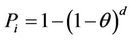
After the direction and concentration of FMDV spread is predicted, probabilities for the infection of farms exposed to airborne virus need to be evaluated. The important factors for the infection are the concentration of airborne virus, the air sampling capacity of the animal, the period of exposure, and the size of the herd. A commonly used concept to consider the risk of infection is the minimum infectious dose. The probability of infection exponentially increases with the size of the dose. The following binomial distribution presents the relationship of the probability (Pi) that an animal is infected when exposed to a given virus dose d in TCID50 and the probability that one TCID50 infects an animal (q) [16]:

(5)

As identified in this study, the probabilities that exposure to one infectious unit (IU) of virus would result in infection, estimated for cattle, sheep, and pigs, are 0.031, 0.045, and 0.003 respectively. Further from Pi, the probability that a group of animals becomes infected (Ph) also depends on the group size (n), given by:

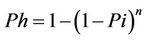(6)

In the case that more than one species is exposed to FMDV for multiple days, more factors must be considered, i.e. species (i), day (k), exposure dose (d), and number of animals of that species on the farm (n) as shown in the following relationship.

(7)

Based on these probabilities, Equations (5)-(7), a relative risk ranking—high, medium, low and very low— can be applied corresponding to probabilities of infection of >50, 10 - 50, 1 - 10 and <1%, respectively.

5. Interpretation of Dispersion Modelling Results

In risk assessment of FMD epidemics via wind-borne spread, reliable techniques and information are very necessary. Whenever possible, data based on actual records during the period of infection must be used. However, sometimes available data relies on estimations such as the exact date of lesions on infected animals, while sometimes it must rely on published values with limitations, which causes imperfection in the prediction [16, 38]. Numerical data producing a worst-case scenario can be optional to guarantee an action plan responding to an outbreak [26]. Consequently, output may be the value expressed as a maximum concentration for a short period, from one hour up to the entire emission period [19].

To carefully interpret the dispersion modelling results in order to develop a management plan, all possible incidences should be considered. For that, a sensitivity analysis of modelling results for assessing the potential for wind-borne spread of FMD to variations in key parameters controlling different physical and biological processes is imperative. Example parameters for such analysis from the literature are serotype of FMDV, biological ageing, weather change according to season, value of q or excretion rate, etc. [38].

6. Discussion

The selection of Gaussian or Lagrangian air dispersion models relies mainly on terrain characteristics affecting meteorological conditions. The Gaussian dispersion model provides a good estimation for aerosol spread of FMDV, and has been applied to the study of both short and long-range transmission. However, Gaussian plume or puff models have many restrictions with disregard to influential factors such as topography or changing wind directions. On the contrary, Lagrangian dispersion models can be applied to almost all inhomogeneous and time varying meteorological conditions as well as non-flat terrain. The model provides a more accurate approximation of the airborne spread of FMDV than the Gaussian dispersion model. Nevertheless, the Lagrangian dispersion model is very complex in use and requires a large number of weather input parameters which are timeconsuming and expensive to attain [8,9,39]. In any case, regardless of which type of air dispersion model is used, meteorological information to support the prediction acquired from both actual records and numerical weather prediction models is a serious factor affecting the accuracy of results [19].

7. Conclusion

To assist management of the potential spread of serious disease like FMD in cloven-hoofed animals, prediction models should be able to determine an accurate range and area of outbreak in advance as well as required minimum data can be obtained since error of prediction might cause serious impact. Selection of suitable model is one of the most important factors providing greater confidence in model outputs. Accuracy in the use of any models for the prediction of FMDV spread requires three essential considerations: 1) the amount of virus released into the atmosphere, 2) factors for virus viability, and 3) minimum quantity of virus causing infection. One of the main causes of FMDV infection via airborne transmission, especially for short-distances over land, is the population density of the target farm, as in the outbreaks in the UK in 1981 and Australia in Case study 1 - 2. For long-distance disease infection over the sea, the outbreak of FMD seems to depend on the coincidence of many factors. It is most likely when the following four circumstances are achieved simultaneously; 1) high output of virus predominantly associated with the outbreak of disease from pigs, 2) low dispersion of virus basically due to stable surface air and light winds, 3) high survival of virus mainly dependent on temperature and relative humidity, and 4) large numbers of susceptible livestock, especially for cows exposed to the virus for many hours [17,22]. Air dispersion modelling approaches to forecast the spread of FMDV are the main focus of this paper but to achieve the successful management and control in any outbreak of FMDV, interdisciplinary knowledge on veterinary, virology, epidemiology, and meteorology is required.

8. Acknowledgements

This research is financially supported by Changwon National University in 2011-2012.

REFERENCES

- G. Davies, “Foot and Mouth Disease,” Research in Veterinary Science, Vol. 73, 2002, pp. 195-199. Hdoi:10.1016/S0034-5288(02)00105-4
- E. Domingo, C. Escarmís, E. Baranowski, C. M. RuizJarabo, E. Carrillo, J. I. Núñez and F. Sobrino, “Evolution of Foot-and-Mouth Disease Virus,” Virus Research, Vol. 91, No. 1, 2003, pp. 47-63. Hdoi:10.1016/S0168-1702(02)00259-9
- E. Maradei, “Characterization of Foot-and-Mouth Disease Virus from Outbreaks in Ecuador during 2009-2010 and Cross-Protection Studies with the Vaccine Strain in Use in the Region,” Vaccine, Vol. 29, No. 46, 2011, pp. 8230- 8240. Hdoi:10.1016/j.vaccine.2011.08.120
- J. N. Cooke and K. M. Westover, “Serotype-Specific Differences in Antigenic Regions of Foot-and-Mouth Disease Virus (FMDV): A Comprehensive Statistical Analysis,” Infection, Genetics and Evolution, Vol. 8, No. 6, 2008, pp. 855-863. Hdoi:10.1016/j.meegid.2008.08.004
- P. V. Barnett, R. J. Statham, W. Vosloo and D. T. Haydon, “Foot-and-Mouth Disease Vaccine Potency Testing: Determination and Statistical Validation of a Model Using a Serological Approach,” Vaccine, Vol. 21, No. 23, 2003, pp. 3240-3248. Hdoi:10.1016/S0264-410X(03)00219-6
- N. Longjam, R. Deb, A. K. Sarmah, T. Tayo, V. B. Awachat and V. K. Saxena, “A Brief Review on Diagnosis of Foot-and-Mouth Disease of Livestock: Conventional to Molecular Tools,” Veterinary Medicine International, Vol. 2011, No. 905768, 2011, pp. 1-17. Hdoi:10.4061/2011/905768
- R. P. Kitching, “A Recent History of Foot-and-Mouth Disease,” Journal of Comparative Pathology, Vol. 118, 1998, pp. 89-108. Hdoi:10.1016/S0021-9975(98)80002-9
- D. Mayer, “A Lagrangian Particle Model to Predict the Airborne Spread of Foot-and-Mouth Disease Virus,” Atmospheric Environment, Vol. 42, No. 3, 2008, pp. 466- 479.
- I. Traulsen and J. Krieter, “Assessing Airborne Transmission of Foot and Mouth Disease Using Fuzzy Logic,” Expert Systems with Applications, Vol. 39, No. 5, 2012, pp. 5071-5077. Hdoi:10.1016/j.eswa.2011.11.032
- D. Sharp, “Foot-and-Mouth Epidemic: The Choices,” The Lancet, Vol. 357, No. 9258, 2001, p. 738. Hdoi:10.1016/S0140-6736(00)04181-7
- H. J. Pharo, “Foot-and-Mouth Disease: An Assessment of the Risks Facing New Zealand,” New Zealand Veterinary Journal, Vol. 50, No. 2, 2002, pp. 46-55. Hdoi:10.1080/00480169.2002.36250
- P. V. Barnett and H. Carabin, “A Review of Emergency Foot-and-Mouth Disease (FMD) Vaccines,” Vaccine, Vol. 20, No. 11, 2002, pp. 1505-1514. Hdoi:10.1016/S0264-410X(01)00503-5
- S. Alexandersen, Z. Zhang, A. I. Donaldson and A. J. M. Garland, “The Pathogenesis and Diagnosis of Foot-andMouth Disease,” Journal of Comparative Pathology, Vol. 129, 2003, pp. 1-36. Hdoi:10.1016/S0021-9975(03)00041-0
- S. Robert and J. Gloster, “Foot-and-Mouth Disease: A Review of Intranasal Infection of Cattle, Sheep and Pigs,” The Veterinary Journal, Vol. 177, No. 2, 2008, pp. 159- 168. Hdoi:10.1016/j.tvjl.2007.03.009
- J. Gloster, A. Jones, A. Redington, L. Burgin, J. H. Sø- rensen, R. Turner, M. Dillon, P. Hullinger, M. Simpson, P. Astrup, G. Garner, P. Stewart, R. D’Amours, R. Sellers and D. Paton, “Airborne Spread of Foot-and-Mouth Disease—Model Intercomparison,” The Veterinary Journal, Vol. 183, No. 3, 2010, pp. 278-286. Hdoi:10.1016/j.tvjl.2008.11.011
- M. G. Garner, G. D. Hess and X. Yang, “An Integrated Modelling Approach to Assess the Risk of Wind-Borne Spread of Foot-and-Mouth Disease Virus from Infected Premises,” Environmental Modeling & Assessment, Vol. 11, No. 3, 2006, pp. 195-207. Hdoi:10.1007/s10666-005-9023-5
- J. Gloster, L. P. Smith, W. H. G. Rees, J. D. Gillett, A. I. Donaldson, J. G. Loxam, R. F. Sellers and F. B. Smith, “Forecasting the Airborne Spread of Foot-and-Mouth Disease and Newcastle Disease,” Philosophical Transactions of the Royal Society of London, Vol. 302, No. 1111, 1983, pp. 535-541. Hdoi:10.1098/rstb.1983.0073
- W. M. Miller, “A State-Transition Model of Epidemic Foot-and-Mouth Disease,” New Techniques in Veterinary Epidemiology and Economics, ISVEE 1, 1976, pp. 56-72.
- J. Gloster, I. Esteves and S. Alexandersen, “Moving towards a Better Understanding of Airborne Transmission of FMD,” Proceedings of the Session of the Research Group of the Standing Technical Committee of the European Commission for the Control of Foot-and-mouth Disease, Rome, 11-15 October 2004, pp. 227-231.
- B. Durand and O. Mahul, “An Extended State-Transition Model for Foot-and-Mouth Disease Epidemics in France,” Preventive Veterinary Medicine, Vol. 47, No. 1-2, 2000, pp. 121-139. Hdoi:10.1016/S0167-5877(00)00158-6
- T. Kostova-Vassilevska, “On the Use of Models to Assess Foot-and-Mouth Disease Transmission and Control,” US Department of Homeland Security Advanced Scientific Computing Program, Lawrence Livermore National Laboratory University of California, Livermore, California, 2004. https://people.ifm.liu.se/unwen/DHS_09/literature/DHS%20report%20FMD%20models.pdf
- R. M. Cannon and M. G. Garner, “Assessing the Risk of Wind-Borne Spread of Foot-and-Mouth Disease in Australia,” Environment International, Vol. 25, No. 6, 1999, pp. 713-723. Hdoi:10.1016/S0160-4120(99)00049-5
- CFSPH, “Foot and Mouth Disease: Fiebre Aftosa,” The Center for Food Security and Public Health, Iowa State University, Iowa, 2007. http://www.cfsph.iastate.edu/Factsheets/pdfs/foot_and_mouth_disease.pdf
- T. Mikkelsen, S. Alexandersen, P. Astrup, H. J. Champion, A. I. Donaldson, F. N. Dunkerley, J. Gloster, J. H. Sørensen and S. Thykier-Nielsen, “Investigation of Airborne Foot-and-Mouth Disease Virus Transmission during Low-Wind Conditions in the Early Phase of the UK 2001 Epidemic,” Atmospheric Chemistry and Physics, Vol. 3, No. 1, 2003, pp. 677-703. Hdoi:10.5194/acpd-3-677-2003H
- F. Moutou and B. Durand, “Modelling the Spread of Foot-and-Mouth Disease Virus,” Veterinary Research, Vol. 25, 1994, pp. 279-285.
- NSW EPA, “Approved Methods for the Modelling and Assessment of Air Pollutants in New South Wales,” Department of Environment and Conservation, Sydney, 2005. http://www.environment.nsw.gov.au/resources/legislation/ammodelling05361.pdf
- M. Caputo, M. Gimenez and M. Schlamp, “Intercomparison of Atmospheric Dispersion Models,” Atmospheric Environment, Vol. 37, No. 18, 2003, pp. 2435-2449. Hdoi:10.1016/S1352-2310(03)00201-2
- C. H. Bosanquet and J. L. Pearson, “The Spread of Smoke and Gases from Chimneys,” Transactions of the Faraday Society, Vol. 32, 1936, pp. 1249-1263. Hdoi:10.1039/tf9363201249
- B. Sportisse, “Box Models versus Eulerian Models in Air Pollution Modeling,” Atmospheric Environment, Vol. 35, No. 1, 2001, pp. 173-178. Hdoi:10.1016/S1352-2310(00)00265-X
- M. Mohan, T. S. Panwar and M. P. Singh, “Development of Dense Gas Dispersion Model for Emergency Preparedness,” Atmospheric Environment, Vol. 29, No. 16, 1995, pp. 2075-2087. Hdoi:10.1016/1352-2310(94)00244-F
- S. P. Arya, “Air Pollution Meteorology and Dispersion,” Oxford University Press, Oxford, 1999.
- G. F. Mackereth and M. A. B. Stone, “Veterinary Intelligence in Response to a Foot-and-Mouth Disease Hoax on Waiheke Island, New Zealand,” Proceedings of the 11th International Symposium on Veterinary Epidemiology and Economics, 2006. http://www.sciquest.org.nz/node/63926
- A. K. Luhar and R. E. Britter, “A Random Walk Model for Dispersion in Inhomogeneous Turbulence in a Convective Boundary Layer,” Atmospheric Environment, Vol. 23, No. 9, 1989, pp. 1911-1924. Hdoi:10.1016/0004-6981(89)90516-7
- S. G. Gopalakrishnan and M. Sharan, “A Lagrangian Particle Model for Marginally Heavy Gas Dispersion,” Atmospheric Environment, Vol. 31, No. 20, 1997, pp. 3369-3382.
- G. Katul, R. Oren, D. Ellsworth, C. Hsieh, N. Phillips and K. Lewin, “A Lagrangian Dispersion Model for Predicting CO2 Sources, Sinks, and Fluxes in a Uniform Loblolly Pine (Pinus taeda L.) Stand,” Journal of Geophysical Research, Vol. 102, No. D8, 1997, pp. 9309-9321. Hdoi:10.1029/96JD03785
- M. Schorling, “Lagrangian Dispersion Model and Its Application to Monitor Nuclear Power Plants,” Environmental Science and Pollution Research, Vol. 2, No. 2, 1995, pp. 105-106. Hdoi:10.1007/BF02986731
- R. R. Draxler, “Hybrid Single-Particle Lagrangian Integrated Trajectory Model,” National Oceanic and Atmospheric Administration, Hysplit PC Training Seminar, 2004. http://www.arl.noaa.gov/documents/workshop/hysplit1/english/workshop.pdf
- G. D. Hess, M. G. Garner and X. Yang, “A Sensitivity Analysis of an Integrated Modelling Approach to Assess the Risk of Wind-Borne Spread of Foot-and-Mouth Disease Virus from Infected Premises,” Environ Model Assess, Vol. 13, No. 2, 2008, pp. 209-220. Hdoi:10.1007/s10666-007-9097-3
- S. Åberg, “Wave Intensities and Slopes in Lagrangian Seas,” Advances in Applied Probability, Vol. 39, No. 4, 2007, pp. 1020-1035. Hdoi:10.1239/aap/1198177237