Atmospheric and Climate Sciences
Vol.3 No.4(2013), Article ID:37964,10 pages DOI:10.4236/acs.2013.34058
On the Downscaling of Meteorological Fields Using Recurrent Networks for Modelling the Water Balance in a Meso-Scale Catchment Area of Saxony, Germany
1Technische Universität Dresden, Dresden, Germany
2Bauman Moscow State Technical University, Moscow, Russia
Email: *rico.kronenberg@tu-dresden.de
Copyright © 2013 Rico Kronenberg et al. This is an open access article distributed under the Creative Commons Attribution License, which permits unrestricted use, distribution, and reproduction in any medium, provided the original work is properly cited.
Received July 31, 2013; revised August 28, 2013; accepted September 5, 2013
Keywords: Downscaling; Recurrent Neural Networks; NARX; WaSim-ETH; Water Balance; ERA-40 Re-Analysis
ABSTRACT
In this study, recurrent networks to downscale meteorological fields of the ERA-40 re-analysis dataset with focus on the meso-scale water balance were investigated. Therefore two types of recurrent neural networks were used. The first approach is a coupling between a recurrent neural network and a distributed watershed model and the second a nonlinear autoregressive with exogenous inputs (NARX) network, which directly predicted the component of the water balance. The approaches were deployed for a meso-scale catchment area in the Free State of Saxony, Germany. The results show that the coupled approach did not perform as well as the NARX network. But the meteorological output of the coupled approach already reaches an adequate quality. However the coupled model generates as input for the watershed model insufficient daily precipitation sums and not enough wet days were predicted. Hence the long-term annual cycle of the water balance could not be preserved with acceptable quality in contrary to the NARX approach. The residual storage change term indicates physical restrictions of the plausibility of the neural networks, whereas the physically based correlations among the components of the water balance were preserved more accurately by the coupled approach.
1. Introduction
Information density and calculation speed of global circulation models (GCM) are highly dependent on the considered spatial and temporal resolution. The resulting contradiction could be solved by different downscaling approaches. Here two major approaches can be distinguished, complex (dynamic) and conceptual (statistic) methods [1]. Dynamic approaches solve the primitive equations with higher temporal and at higher spatial resolution with higher resolved and better parameterized processes and use the GCM output as initial and boundary conditions. Often more than one nesting step is used, like in REMO [2,3], CLM [4] or WRF [5], where the previous nesting step delivered the initial and boundary conditions for the current nesting step of the considered domain.
Instead stastistic approaches are less computational demanding. Reference [6] compared in one of the first summaries of stastistic downscaling approaches different methods for single sites. They divided the approaches into three categories: 1) Regression methods; 2) Weather pattern based methods; 3) Stochastic generators. Generally they concluded that pattern based approaches perform best on daily basis but were restricted to the quality of GCM data. This restriction refers to a strict dependency of GCM derived weather patterns and downscaled climate variables. Reference [7] noted different categorization of stastistic methods. They divided empirical downscaling into linear and non-linear regression, artificial neural networks (ANN), canonical correlation and principle component analysis. In their study they compared a recurrent neural network (i.e. temporal neural network) with a regression approach for the downscaling of minimum, maximum temperature and precipitation and found that the ANN results reproduced the observed extremes in adequate quality, which is not necessarily the case for the unobserved future values. Reference [8] used an artificial neural network to downscale hourly 27 km spaced precipitation fields of mesoscale model 5 (MM5) output to hourly 3 km spaced fields. They obtained their best results under consideration of elevation, the relations to neighbouring grid cells and time components as predictors. Predictors derived from GCM output and the considered domain play an important role, which [9] deeply investigated. They developed a scheme to optimize, by simulated annealing, the necessary number of predictors and their 3-dimensional domain for single sites to downscale precipitation by means of an ANN approach. Their results showed a strong dependency of climate variable and predictor domain, which can differ from climate variable to climate variable. But until now ANNs have not been applied in the modelling of climate datasets for the study region of Saxony. The major question was how do ANNs perform in the context of a water balance model (i.e. the driving input of the water balance model is the ANN output) or to downscale the water balance of a meso-scale catchment area directly. This question arises, precisely because the generated local meteorological information is often used as further input for another model. This study aims to answer the following questions:
Ÿ How large are the quantitative differences between modelled and observed water balance in a meso-scale catchment area?
Ÿ How consistent are the resulting dataset in terms of physically based correlations among the elements of the water balance?
Ÿ Do ANNs prevent the long-term annual cycle of the water balance?
To answer these questions two approaches using different kinds of recurrent neural networks are presented.
2. Data
2.1. Catchment Area and Hydrological Data
The study region is the catchment area of the Zschopau River, which wells in the Ore Mountains and flows into the Freiberger Mulde River. The study region is depicted in Figure 1. The catchment is characterized by a large percentage of mountains that is the reason why here the coldest average temperature (1961-1990) of Saxony can be found. The average temperature ranges from <4˚C in the ridges of the mountains to 8˚C in the valleys of the catchment area. Furthermore in the catchment can be observed a comparable large variability in the annual precipitation amount from 750 mm in the valleys to >1200 mm in the mountain ranges (i.e. mean annual precipitation sums from 1961 to 1990) [10]. The whole catchment reaches from the middle Ore Mountains and the eastern Ore Mountains to the Mulde River and Ore Mountain valleys [11]. The gauging station for the catchment area is Kriebstein, which is located 14.4 km downstream of the Zschopau River and measures the

Figure 1. Catchment area of the Zschopau River with rain gauges and climate stations; the catchment lies in the eastern part of Germany, in the south of the federal state of Saxony and covers a large part of the Ore mountains.
discharge for a 1757 km2 large area. The gauging station Kriebstein is located downstream behind the dam Kriebstein and is operated by the State Reservoir Administration of Saxony. Thus more or less meaningful influence can be observed at the gauging station through manipulated discharge and flood behaviour of the river.
2.2. Meteorological Data
The daily observed meteorological variables for the study region were measured by the monitoring network of the German weather service (DWD) and the Czech hydrological-meteorological service (CHMI). The data were processed by the Saxonian climate database CLISAX [12-15], where also the quality assessment of the series was done. The deployed elements are summarized in Table 1, which are the minimum input variables for the distributed water balance model WaSim-ETH [16]. Hence, the choice of stations which were appropriate for the water balance simulations are limited by the catchment area of the Zschopau River.
Besides all stations within the catchment also time series of neighbouring stations were used (cp. Figure 1) aiming as much dens information as possible for the spatial interpolation of the meteorological fields. Overall 68 daily precipitation gauges and 19 climate stations of the DWD and CHMI were available for the downscaling and water balance modelling within the period from 1975 to 2000. The meteorological fields are summarized in Table 1, which were deployed as predictor variables. The
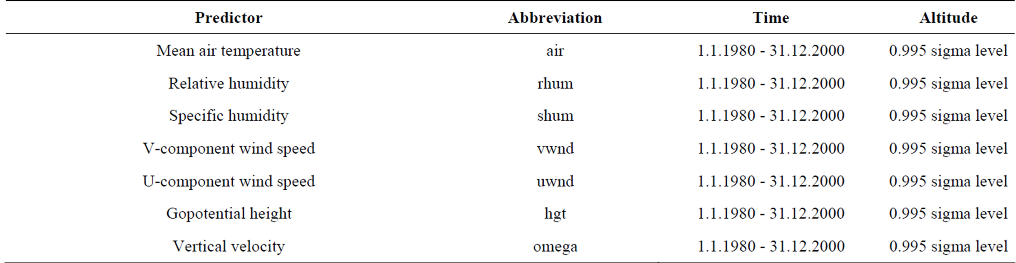
Table 1. Used daily predictor variables derived from the ERA-40 re-analysis data set.
ERA-40 re-analysis data set was described in [15]. Fields were extracted with the bounding box of the shown territory in Figure 1, which resulted into four grid cells with a spatial resolution of about 125 km (i.e. 2.5˚).
3. Methods
3.1. Water Balance Modelling with WaSim-ETH
For the modelling of the water balance the distributed model WaSim-ETH was applied. This modelled was developed by [16] at the ETH Zurich and modified by [14]. The model enables the user to calculate grid and physically based the components of the water balance with high spatial and temporal resolution. The model is module based, which allows the user to change specific modules and adapt them for certain questions or investigations. A detailed description of the modules can be found in [14,16] and further adaptations of the model in [17,18].
For the simulation of the water balance the model needs information of the initial state of the ground storage. If no or just uncertain information is delivered it is recommended to considered the first 2 to 5 years as warming-up period in the model. The model was applied in its WaSim-ETH 7.10.1 version with unsaturated homogeneous soil column and a Richards approach. It has to be mentioned that the model underlies a steady development process. The model calibration with focus on the long term discharge was done by the automatic parameter estimation and calibration software PEST [19]. The optimization scheme was applied for a non linear identification of spatially distributed sets of parameters.
3.2. Hydrological Performance Indices
The Nash-Sutcliff efficiency (NSE) is a statistical performance index to calculate the relative difference between a simulated (Ysim) and an observed series (Yobs). The index shows how close the data curve lies to the 1:1 line. The NSE ranges from −∞ to 1, where 1 means the best relation between observed and simulated data. Reference [20] stated that the NSE is the best performance index to evaluate hydrological models. It is defined in Equation (1).
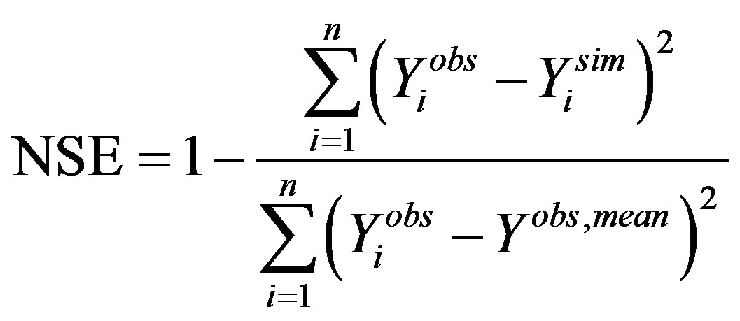 (1)
(1)
The RMSE was deployed to calculate the mean daily deviations of the simulated to the observed discharge. The smaller the RMSE the better fit the model results the observed states. Following [21] also a normalized RMSE was used, standardized by the standard deviation (RSR). RSR ranges from 0 to +∞. The closer the RSR lies to 0 the better the daily simulated values fit the observed discharges. The RMSE can be calculated following Equation (2).
 (2)
(2)
The percent BIAS describes the mean relative difference of the simulated series to the observed discharge series in percentages over the whole observation period. It is calculated as defined in Equation (3). A 1-to-1 relation is characterized through a PBIAS of 0.0%. Positive values mean that the hydrological model overestimates the discharge and a negative PBIAS an underestimation. Reference [20] gave the following ranges and qualities for the performance indices on monthly basis to evaluate hydrological models. The ranges can be found in Table 2. The model calibration with focus on the discharge should therefore aim for a good to very good performance according to these indices.
 (3)
(3)

Table 2. Hydrological performance indices and their quality related to monthly calculated discharge [20] .
3.3. Neural Networks for the Downscaling Task
Applied in this study were neural networks which belong to the group of recurrent neural networks (RNN) [22]. The first network is a pseudo recurrent neural network (PRNN) as described in [7] (i.e. time lagged feed-forward neural network) and the second a nonlinear autoregressive with exogenous inputs (NARX) network [23].
The studied PRNN was adapted and applied in the following manner. The differences to a simple multilayer feed forward network lays in the input layer which contains not just the actual but also time lagged values. This enables the network to learn a pseudo memory, since a part of the weights were adjusted for the past states of the system. In this case the pseudo memory could be the past state of the atmosphere of a defined period (between 1 to 10 days). Potential predictors could be found in [6-9]. These are passed, through weights, to the hidden layers, which are hierarchically connected to each other. The output layer represents the cumulative theoretical probabilities (CDF) of the in Table 3 mentioned climate variables for all considered stations.
Neural networks are often mentioned in the context of non linear systems [24,25]. NARX models are useful models to predict discrete dynamic time series. The applied theory for the used NARX network can be found in [26]. The exogenous input was defined as the predictor variables derived from the ERA-40 re-analysis data (cp. Table 1). In contrast to the PRNN the NARX was particularly applied for each component of the water balance (cp. Equation (4)). The network was deployed in an open-loop for the training and in closed-loop mode for the final predictions.
In behalf of the approximation theorem [27] just networks with one single hidden layer were used for downscaling. Neural networks are considered as robust against noise, though potential uncertainties have to be mentioned. The main disadvantage with in the networks might be the latent risk of finding just local minimums of the energy function used for the weights adaption and network training. Also the problem of over fitting may occur. Further uncertainties may arise through the data generalization by the description by parametric distribution functions (cp. Table 3).
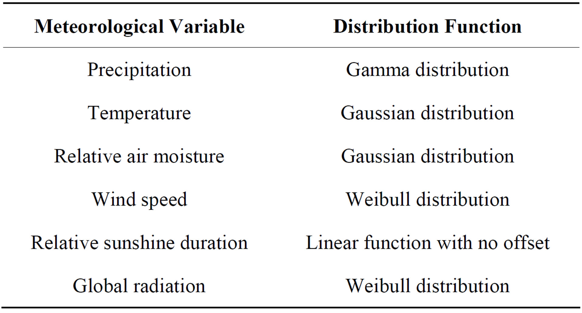
Table 3. Chosen CDFs for the parametric modeling of the distribution of meteorological variables in daily resolution for stations in and around the catchment area of Zschopau River [28-30].
The two approaches and their necessary input data for the modelling the water balance are summarized in the scheme in Figure 2. As can be seen for the NARX model no DWD data was used instead the network was trained directly to the WaSim-ETH output.
4. Results and Discussion
The main focus of this study lies in the downscaling of meteorological fields and their impact on the long term water balance. Hence the results have to be validated in terms of meteorological and hydrological qualities. Meteorological properties are analyzed element wise by considering their positive extremes (i.e. quantiles). Hydrologically the interpretation focused on the in Equation (4) defined long-term water balance in its most common and most simple form. Precipitation (P) is the sum of the discharge (Q), the evapotranspiration (E) and the storage change (dS). More detailed investigations of governing sub processes are neglected.
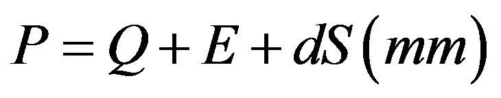 (4)
(4)
4.1. WaSim-ETH Calibration and Validation
The calibration of WaSim-ETH for the Zschopau River was done for the complete data set (i.e. all available stations). Therefore the time series were divided into a calibration (from 01.01.1994 to 31.12.1999) and a validation data set (from 01.01.1980 to 31.12.1990). The iterative calibration procedure by PEST optimized the parameters according to the discharge. The results are shown in Table 4. Obviously the parameter optimization by PEST resulted in good performances in terms of hydrological quality measures for daily resolution. The NSE as well as RSR and PBIAS lie in the area of a very good performance (cp. Table 2). For the validation a decrease of the performances measures was expected, as the validation is the assessment how the model performs for unobserved states. Except of PBAIS, the simulations in terms of NSE and RSR slightly lose their good performance, though still reach good results. WaSim-ETH was used in this configuration. No further adaption of the parameters was done. The hydrological qualities of the modelled discharge over the whole available time period are summarized in Table 4. The model was driven by the complete set of available meteorological stations (MODF) and by a reduced set (MODS). This reduction is meant in terms of expelling stations within the observed period, which include daily defaults. Hence really complete series were used for the MODS runs. Explicitly this reduction meant a shrinking from 68 to 31 precipitation gauges and 19 to 6 climate stations within and around the catchment area. The MODF run is quite close to a very good performance in the period from 01.01.1980 to 31.12.1999. Yet the MODS run just achieved an acceptable quality due to the
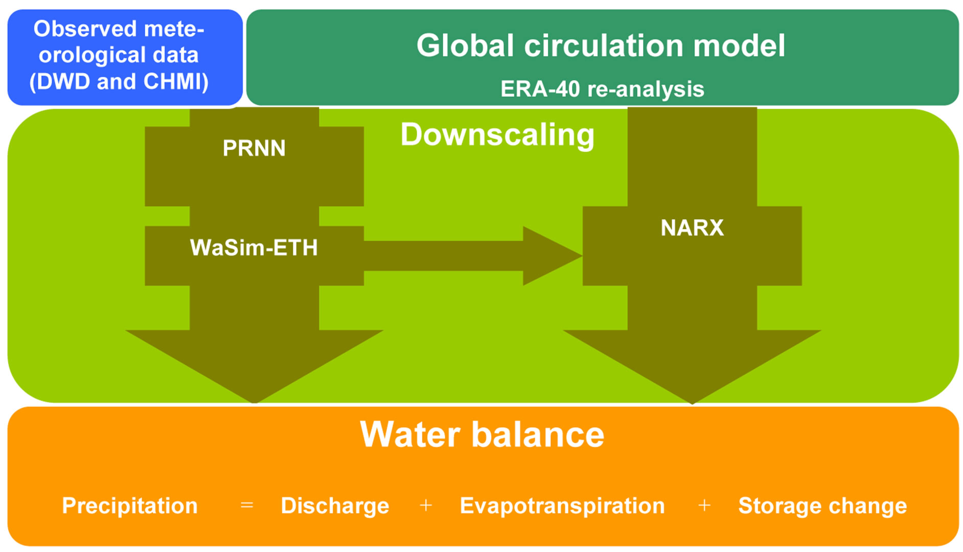
Figure 2. Downscaling scheme: How to come from global model data to a local water balance, two approaches were distinguished: first a coupling of a PRNN and a distributed watershed model (WaSim-ETH) and second a NARX model.

Table 4. Hydrological quality measures on daily modeled discharge for different runs and periods.
reduced meteorological input. Attempts to calibrate the model for the reduced meteorological series did not successfully lead to good results of the modelled discharge. Thus WaSim-ETH was utilized for the calibrated version with full meteorological input driven by a reduced dataset.
4.2. Neural Network Training
The training for the recurrent networks resulted for all configurations into good results in terms of the regression coefficient R. In Table 5, the results can be seen. The naming of each realization is defined as follows; first the days of delay (i.e. time lagged days) and second the number of neurons in the hidden layer. As regression coefficient R indicates for the validation and test datasets the networks are not over-fitted, since any of these configurations are really close to the trained dataset. The validation and test datasets were randomly generated each contained 15% of all available days. According to R each realization can be considered as satisfied approximation of the observed data. Best results show the PRNN_3_80 and PRNN_5_80 realizations with 0.81 in the training mode, worst can be found in the PRNN_0_20 with 0.76.

Table 5. Neural network performance (regression coefficient R) after training over the period from 01.01.1980 until 31.12.1999, the dataset was randomly splitted into 70% training, 15% validation and 15% test data.
The training of the NARX network leads to more distinguishable results in terms of R. It clearly can be seen in Table 5 that for precipitation (P) for the short configuration (PS) as well as the full configuration (PF, i.e. full = all stations) just satisfactory qualities of 0.56 and 0.48 for the training data, less 0.35 for the validation and test datasets could be achieved. Using other combinations of predictors even lead to worse results so that using this model (i.e. NARX) and the chosen predictor data no better results could be obtained. Surprisingly good instead performed the discharge (Q) and the evapotranspiration (E), while there are no significant difference in the performance of the short (ES) or full (EF) dataset of the evapotranspiration of 0.86 in the training phase.
4.3. Meteorological Results of the Recurrent Neural Network
The 0.99 quantiles of the meteorological output from the recurrent networks are shown in Figures 3 and 4. Each sample point represents the 0.99 quantile of a specific element at a certain station in the catchment area.
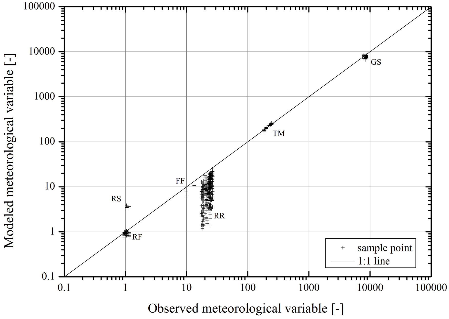
Figure 3. 0.99 quantiles of all realizations and all stations after downscaling with PRNN for precipitation (RR [mm/d]), wind speed at 2 m (FF [m/s]), mean temperature (TM [˚C]), relative sunshine duration (RS [−]), moisture (RF [%]) and global radiation (GS [Wh/m²]).

Figure 4. 0.99 quantiles of all realizations and all stations after downscaling with PRNN for precipitation.
Every element is drawn at the graph. Obviously each element forms a more or less scattered cloud. Despite the wind (FF), as can be seen, the 0.99 quantile is constant over all realizations due to the linear function used for the CDF. The relative humidity (RF) is for all realizations close to 100 %, the mean daily temperature (TM) lies between 17.1˚C and 26.2˚C and the global radiation (GS) around 7500 Wh/m². These four elements compared to the observed quantiles are really close to the 1:1 line. Only the relative sunshine duration (RS) and the precipitation (RR) show significant deviations from the observed values. While RS is consequently over estimated (i.e. 0.99 Quantile) by the neural network for RR an underestimation becomes obvious. However, on the one hand the overestimation of RS seems systematic, since the scattering is limited. For this and physical reasons RS was corrected, in case a value exceed 1 it was reset to 1. On the other hand, the wide scattering of RR does not support the thesis of a systematic underestimation. Hence its deviations seem to be randomly. One reason for the underestimation may be the choice of a rather simple parametric CDF (cp. Table 3), which dos not accurately describes the extremes of precipitation.
4.4. Monthly Mean Water Balance
The hydrological quality measures for the different model runs (i.e. PRNN with WaSim-ETH and NARX) are summarized in Table 6 for monthly values. The best performance could be achieved by the NARX model with an NSE of 0.99. The model performs surprisingly well for the modelled period. Also MODF and MODS (WaSim-ETH driven by observed meteorological input) reached according to [20] a very good quality for NSE, RSR as well as PBIAS in contrast to the recurrent network realizations.
WaSim-ETH driven by the downscaled input could rarely reach satisfactory results on a monthly basis. For example just three realizations have a NSE of larger than 0.30. Also RSR and PBIAS yield poor results for the modelled discharge in the catchment. To find feasible reasons for the modest results also the other components of the water balance have to be taken into account for interpretation.
In Figure 5, the average monthly sums of the water balance components are depicted for all model runs. Area means generated by interpolations were used for the interpretation of the components. Precipitation (cp. Figure 5(a)) with its variability in space and time is a difficult variable for this kind of prediction. The precipitation results from the MODF are defined as standard or in other words as observed. Each other realization of precipitation has to be evaluated by this measure. The MODS results lie closely to the MODF curve, which
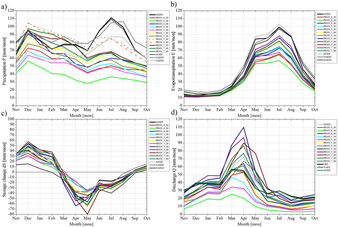
Figure 5. Monthly mean water balance components: (a) Precipitation, (b) Evapotranspiration, (c) Groundwater storage change, (d) Discharge.

Table 6. Hydrological quality measures for monthly modeled discharge for different runs of PRNN with WaSimETH and the NARX model for the period 01.01.1980 to 31.12.1999.
indicates that for precipitation over area the impact of the reduction of gauging stations is rather small. The most similarities in the annual cycle of precipitation could be achieved by the NARXF and NARXS results.
Interesting are the significant underestimation which occurred by reducing the gauge density in the catchment area. This indicates that there might by significant differences in the daily precipitation which are smoothed by monthly means. These differences of the precipitation over area have a stronger impact on the downscaling by NARX than on the spatial averaging. Going back to the similarities of the annual curve the bimodal character of the observed state almost could be achieved with two peaks. One peak in December and one even stronger one in the summer around the month July and August are apparent, which cover with observations in the catchment [31].
The MODF run shows a deviant behaviour compared with the different configurations of the recurrent network. They all have a similar annual cycle of precipitation often with two peaks. But the stronger peak always occurs in winter. While winter and spring closely behave like the MODF run the summer shows significant differences in terms of underestimation. In general an underestimation of precipitation can be observed. Taking into account the underestimation of single days (cp. Figures 3 and 4) it must be stated that for single days insufficient precipitation sums are computed and an insufficient number of wet days are generated by PRNN compared to observations.
The curves of evapotranspiration over area show independent of the model run similarities. The differences just lie in the amount of water. The annual cycle was conserved by each model run. The systematic underestimation for especially the PRNN runs could easily be explained by the shortage of available water particularly in the summer months. Underestimations of precipitation by the recurrent network compulsorily lead to a systematic underestimation of transpirated water, which clearly can be seen in Figure 5(b). The peak can be found in the summer, since the energy input over the catchment is at its maximum. The discharge as output of the hydrological system concludes the main component of the budget. The annual cycle is similar in all runs. The highest discharge can be found in spring after the melting of snow. In summer it is small because of the large evapotranspiration. Regarding the rather large precipitation values of the PRNN runs in winter and the underestimated evaporation results in the winter lead to significant peaks in April, which obviously are largely overestimated. In summer, the discharge is underestimated by the PRNN due to the underestimated precipitation in this period. The storage change as residual of the water balance shows for all runs a less variable annual cycle with increasing amount of water stored in the winter in the form of ice and snow and a negative term in summer caused by the large amount of available water which evaporates.
4.5. Yearly Mean Water Balance
The yearly means of the water balance components are summarized in Table 7. For the recurrent network runs a general trend of underestimation is obvious. The large percentage deviation of the storage change seems to be dramatic. But it is not, since the absolute value of dS is comparatively small to the other components.
But 10% and more have to be mentioned, which mainly occur because of the poor precipitation estimation. For the recurrent network runs PRNN_5_40 and PRNN_5_80 seems the most suitable yet not satisfactory, comparing them to the really good bias of less than 1% of the NARX model especially for Q. But also the bias of P and E for NARXF and NARXS are satisfactory in contradiction to dS which exceed a multiple of the observed value. Yet this exceedance may be expected since the absolute average value of dS plays a marginal role in the catchment area. The absolute yearly mean values for the water balance are drawn in Fig-

Figure 6. Yearly mean water balance components: P = Precipitation, E = Evapotranspiration, Q = Discharge; PRNN is depicted with all realizations, the different runs of PRNN are summarized.

Table 7. Annual bias of water balance components from the absolute observed values for the model runs.
ure 6. As can be seen the biggest differences between the model runs can be found in the precipitation. The realizations of the recurrent network are summarized and reach from 500 mm to not much more than 1000 mm, while NARXF lays close to the observed sum the NARXS underestimates it significantly. The best yearly result achieved NARXF followed by NARXS for E and Q as already shown in Table 7, the deviations are marginal.
5. Conclusions and Outlook
By now downscaled meteorological data are already used in practical applications. There often the question arises about the quality of the downscaled data, precisely because the input data governs the quality of the specific application output. In this study this application was the modelling of a meso-scale water balance. Two approaches were deployed for a representative catchment area of the Free State of Saxony, Germany. The approaches belong to a group of recurrent neural networks. First a coupled approach was implemented and investigated with a recurrent neural network and a watershed model and second a NARX network to downscale meteorological fields of the ERA-40 re-analysis dataset. The findings show that recurrent networks should be used carefully for downscaling climate elements, especially precipitation. Explicitly the underestimation of daily sums and the underestimation of the number of wet days by the coupled approach are main problems, significantly influencing the results of the water balance model. The findings confirm the known weaknesses of stochastic downscaling approaches by producing rather fuzzy information of discrete variables like precipitation. A coupling of ANN with Markov chain models [32] and a better functional description of precipitation CDFs through mixture distributions [33] or non-parametric distributions [34] may lead to better results.
Apart from that, the downscaling process lead to more consistent data, which can be seen in the residual storage change term in contrast to the NARX runs. The bias is significantly smaller than for NARX which exceed the observed storage change multiple times and indicates a smaller consistency for the climate variables of a daily resolution. But the hydrological quality measures as well as the monthly and yearly outputs speak for the use of NARX models to simulate the water balance for a mesoscale catchment area. Likewise the application is less time and knowledge demanding.
6. Acknowledgements
This work was supported by the Erasmus Mundus Action 2 Programme of the European Union and the German Weather Service (DWD) and the Czech HydrologicalMeteorological Service (CHMI). R.K. likes to thank Dr. Yana Kinderknecht from the Chair of Mathematical Modelling for the kind supervision at BMSTU in 2012/ 2013.
REFERENCES
- H. von Storch, S. Güss and M. Heimann, “Das Klimasystem und seine Modellierung—Eine Einführung,” Springer-Verlag, Berlin, Heidelberg, 1999. http://dx.doi.org/10.1007/978-3-642-58528-9
- D. Jacob, “A Note to the Simulation of the Annual and Inter-Annual Variability of the Water Budget over the Baltic Sea Drainage Basin,” Meteorological Atmospheric Physics, Vol. 77, 2001, pp. 61-73. http://dx.doi.org/10.1007/978-3-642-58528-9
- D. Jacob, H. Göttel, S. Kotlarski, P. Lorenz and K. Sieck, “Klimaauswirkungen und Anpassung in Deutschland— Phase 1: Erstellung Regionaler Klimaszenarien für Deutschland,” 2008.
- H. D. Hollweg, U. Böhm, I. Fast, B. Hennemuth, K. Keuler, E. Keupthiel, M. Lautenschlager, S. Legutke, K. Radtke, B. Rockel, M. Schubert, A. Will, M. Woldt and C. Wunram, “Ensemble Simulations over Europe with the Regional Climate Model CLM Forced with IPCC AR4 Global Scenarios,” M & D Technical Report 3, 2008.
- W. C. Skamarock, J. B. Klemp, J. Dudhia, D. O. Gill, D. M. Barker, M. G. Duda, X. Huang, W. Wang and J. G. Powers, “A Description of the Advanced Research WRF Version 3,” NCAR Technical Note June 2008, 2008.
- R. L. Wilby and T. M. L. Wigley, “Downscaling General Circulation Model Output: A Review of Methods and Limitations,” Progress in Physical Geography, Vol. 21, No. 4, 1997, pp. 530-548. http://dx.doi.org/10.1177/030913339702100403
- Y. B. Dibike and P. Coulibaly, “Temporal Neural Networks for Downscaling Climate Variability and Extremes,” Neural Networks, Vol. 19, No. 2, 2006, pp. 135- 144. http://dx.doi.org/10.1016/j.neunet.2006.01.003
- B. Tomassetti, M. Verdecchia and F. Giorgi, “NN5: A Neural Network Based Approach for the Downscaling of Precipitation Fields—Model description and preliminary results,” Journal of hydrology, Vol. 367, No. 1-2, 2009, pp. 14-26. http://dx.doi.org/10.1016/j.jhydrol.2008.12.017
- T. Sauter and V. Venema, “Natural Three-Dimensional Predictor Domains for Statistical Precipitation Downscaling,” Journal of Climate, Vol. 24, No. 23, 2011, pp. 6132-6145. http://dx.doi.org/10.1175/2011JCLI4155.1
- C. Bernhofer, V. Goldberg, J. Franke, J. Häntschel, S. Harmansa, T. Pluntke, T. Geidel, M. Surke, H. Prasse, E. Freydank, S. Häsel, U. Mellentin and W. Küchler, “Sachsen im Klimawandel—Eine Analyse,” Sächsisches Staatsministerium für Umwelt und Landwirtschaft, Dresden, 2008, p. 211.
- K. Mannsfeld, O. Bastian, A. Kaminski, W. Katzschner, M. Röder, R.-U. Syrbe and B. Winkeler, “Landschaftsgliederungen in Sachsen,” Mitteilungen des Landesvereins Sächsischer Heimatschutz e.V., Sonderheft, Dresden, 2005, p. 68.
- C. Bernhofer and V. Goldberg, “CLISAX—Statistische Untersuchungen Regionaler Klimatrends in Sachsen,” TU Dresden, Institut für Hydrologie und Meteorologie, 2001.
- J. Franke, V. Goldberg, U. Eichelmann, E. Freydank and C. Bernhofer, “Statistical Analysis of Regional Climate Trends in Saxony, Germany,” Climate Research, Vol. 27, No. 2, 2004, pp. 145-150. http://dx.doi.org/10.3354/cr027145
- J. Schulla and K. Jasper, “Model Description WaSiM- ETH,” Internal Report, Institute for Atmospheric and Climate Science, ETH Zürich, 2007, p. 181.
- S. M. Uppala, P. W. Kållberg, A. J. Simmons, U. Andrae, V. da Costa Bechtold, M. Fiorino, J. K. Gibson, J. Haseler, A. Hernandez, G. A. Kelly, X. Li, K. Onogi, S. Saarinen, N. Sokka, R. P. Allan, E. Andersson, K. Arpe, M. A. Balmaseda, A. C. M. Beljaars, L. van de Berg, J. Bidlot, N. Bormann, S. Caires, F. Chevallier, A. Dethof, M. Dragosavac, M. Fisher, M. Fuentes, S. Hagemann, E. Hólm, B. J. Hoskins, L. Isaksen, P. A. E. M Janssen, R. Jenne, A. P. McNally, J.-F. Mahfouf, J.-J. Morcrette, N. A. Rayner, R. W. Saunders, P. Simon, A. Sterl, K. E. Trenberth, A. Untch, D. Vasiljevic, P. Viterbo and J. Woollen, “The ERA-40 Re-Analysis,” Quarterly Journal of the Royal Meteorological Society, Vol. 131, No. 612, 2005, pp. 2961-3012. http://dx.doi.org/10.1256/qj.04.176
- J. Schulla and K. Jasper, “Modellbeschreibung WaSiMETH,” Technischer Bericht, Institut für Atmosphäre und Klima, ETH Zürich, 1998, p. 152.
- J. Scherzer, G. Wriedt, D. Sames, M. Müller, F. Hesser, K. Jasper and H. Pöhler, “KLiWEP—Abschätzung der Auswirkungen der für Sachsen Prognostizierten Klimaveränderungen auf den Wasserund Stoffhaushalt im Einzugsgebiet der Parthe—Teil 3: Vorstudie zur Simulation der Stoffflüsse von Stickstoff und Kohlenstoff im Parthe-Einzugsgebiet,” 2006.
- H. Pöhler, F. Chmielewski, K. Jasper, Y. Hennings and J. Scherzer, “KliWEP -Abschätzung der Auswirkungen der für Sachsen Prognostizierten Klimaveränderungen auf den Wasserund Stoffhaushalt im Einzugsgebiet der Parthe—Weiterentwicklung von WaSiM-ETH: Implikation Dynamischer Vegetationszeiten und Durchführung von Testsimulationen für Sächsische Klimaregionen,” Sächsisches Landesamt für Umwelt und Geologie, Abschlussbericht des Forschungsund Entwicklungsvorhabens Nr. 13, 2007.
- J. Doherty, “Model-Independent Parameter Estimation User Manual: 5th Edition,” Watermark Numerical Computing, 2004, p. 336.
- D. N. Moriasi, J. G. Arnold, M. W. Van Liew, R. L. Bingner, R. D. Harmel and T. L. Veith, “Model Evaluation Guidelines for Systematic Quantification of Accuracy in Watershed Simulations,” Transactions of the ASABE, Vol. 50, 2007, pp. 885-900.
- J. Singh, H. V. Knapp, J. G. Arnold and M. Demissie, “Hydrologic Modeling of the Iroquois River Watershed Using HSPF and SWAT,” Journal of the American Water Resources Association, Vol. 41, No. 2, 2005, pp. 343-360. http://dx.doi.org/10.1111/j.1752-1688.2005.tb03740.x
- T. Jayalakshmi and A. Santhakumaran, “Statistical Normalization and Back Propagation for Classification,” International Journal of Computer Theory and Engineering, Vol. 3, No. 1, 2011, pp. 89-93. http://dx.doi.org/10.7763/IJCTE.2011.V3.288
- C. Jiang and F. Song, “Sunspot Forecasting by Using Chaotic Time Timeseries Analysis and NARX Network,” Journal of Computers, Vol. 6, No. 7, 2011, pp. 1424- 1429. http://dx.doi.org/10.4304/jcp.6.7.1424-1429
- C. M. Bishop, “Neural Networks for Pattern Recognition,” Oxford University Press, 1996, p. 482.
- J. M. P. Menezes Jr. and G. A. Barreto, “Long-Term Time Series Prediction with the NARX Network: An Empirical Evaluation,” Neurocomputing, Vol. 71, No. 16-18, 2008, pp. 3335-3343. http://dx.doi.org/10.1016/j.neucom.2008.01.030
- H.-Y. Shen and L.-C. Chang, “Online Multistep-Ahead Inundation Depth Forecasts by Recurrent NARX Networks,” Hydrology and Earth System Sciences, Vol. 17, 2013, pp. 935-945. http://dx.doi.org/10.5194/hess-17-935-2013
- S. Haykin, “Neural Networks and Learning Machines,” 3rd Edition, Pearson Prentice Hall, Upper Saddle River, 2009.
- H. von Storch and F. W. Zwiers, “Statistical Analysis in Climate Reasearch,” Cambridge University Press, 2010.
- D. S. Wilks, “Statistical Methods in the Atmospheric Sciences: An Introduction,” International Geophysics Series, Vol. 59, Academic Press, 1995, p. 464.
- C.-D. Schönwiese, “Praktische Statistik für Meteorologen und Geowissenschaftler,” 4 Auflage, Verlag Gebrüder Borntraeger, Stuttgart, 2006, p. 302.
- C. Bernhofer, J. Matschullat and A. Bobeth (Hrsg.), “Das Klima in der Modellregion Dresden,” Rhombos-Verlag, Berlin, 2009, p. 117.
- D. S. Wilks and R. L. Wilby, “The Weather Generation Game: A Review of Stochastic Weather Models,” Progress in Physical Geography, Vol. 23, No. 3, 1999, pp. 329-357. http://dx.doi.org/10.1177/030913339902300302
- R. Kronenberg, J. Franke and C. Bernhofer, “Comparison of Different Approaches to Fit Log-Normal Mixtures on Radar-Derived Precipitation Data,” Meteorological Applications, 2013, I press. http://dx.doi.org/10.1002/met.1408
- M. Mudelsee, M. Börngen, G. Tetzlaff and U. Grünwald, “Extreme Floods in Central Europe over the Past 500 Years: Role of Cyclones Pathway, ‘Zugstrasse Vb’,” Journal of Geophysical Research, Vol. 109, No. D23, 2004, pp. 1-21. http://dx.doi.org/10.1029/2004JD005034
NOTES
*Corresponding author.