ABSTRACT

The present paper is of historic importance as well as the second part of [1] . In this second part, we detect important details about the orbit of the Earth and about the velocity (of magnitude 217 km/s) of the solar system around the center of the Milky Way galaxy. Some of these details concern the perihelion and aphelion of the orbit of the Earth. For several years we have observed that the return pulses, on the oscilloscope screen, appear to be more energetic than the initial pulses, see first and second photo of Figure 8 (See, also, Part 1, Figure 2, for which the return pulse crests are much higher than the initial crests). The used oscilloscope is and only must be, a storage oscilloscope, in other words, a computerized oscilloscope with a digital memory. The first oscilloscopes like this, came out, only after 1995, a relatively recent time that all wire velocity experiments and measurements were already completely investigated by science. We do astronomy, without receiving images by an astronomical telescope, but instead by sending signals around a loop and making an analysis using the same oscilloscope as in Part 1. We recommend to the reader to study Part 1 as a prerequisite. The Earth surface is accelerating with a centripetal acceleration, due to its rotation, thus it is not an inertial frame. Also, the Earth is evidently anisotropic, due to the same rotation, a second reason for it being a non-inertial rotating frame.

Keywords:

Inertiality, Isotropy, Anisotropy, Gain of Free Energy, Ether, Energy, Storage, Digital Computerized, Oscilloscope

1. Introduction

The raw data is impossible to be published in any scientific journal as these data consist of more than a total of than 50,000 measurements, recorded by several observations daily during the last several years. These data alone will take several issues of the present or any other journal, to be published. However, it can be available in the website [2] . As explained in the abstract and described in the title, this Part 2 is a continuation of Part 1 with additional details. Part 2 is using a closed loop of 134 meters. Part 2 does not show the daily reversals early in the morning and late in the night, which was shown several years ago, in Part 1. We have been unable to understand and explain this difference between the present years 2017-2018, as compared with the period of observation of Part 1 some years ago. After various trials, we concluded that the best and most enlarged effects were with the longer loop. Based on the availability of our space of our back-yard, we have chosen 134 meters, the longest possible loop. The details and the adequacy of our instrumentation are described in Part 1.

2. Possible Explanations or Not of the Present Observations

Proper and Trivial Explanation of the Magnetic Field of the Earth, Discussion of Pole Reversals

The surface of Earth is known to be charged [3] negatively with 10⁻⁵ Coulombs. Based on this fact and the fact that the Earth effectively is counter-clockwise rotating at an equator speed of 465 m/s, the Earth is producing with respect to this rotation, an effective current. We deduce immediately and very trivially, a magnetic field for the Earth, with a correct magnetic south pole for the north geographic pole and vice versa, avoiding the complicated and difficult to understand theory of the dynamo, which is only hypothetical and without any particular observational evidence. See the easier explanation below.

This is the rigorous crystal clear explanation of magnetic poles’ formation for the earth and also for other planets and for the Sun in our solar system and other stellar systems. As well this presents for the first time a simple and crystal clear explanation of the unexplained by literature poles’ reversals.

The formation of the magnetic poles of Earth is shown in Figure 1, and its written descriptions are in the figure. So, for a complete description of the formation of the magnetic poles of the Earth, see Figure 1 and its caption, which may stand for our Sun and any other planetary system in our Universe.

Farther, we might claim, for now, the Earth’s surface, we know, is negatively charged and as these charges are repelled and distributed on a sphere, then as far as the Coulomb forces go, these charges are equivalent to as if they were all concentrated at the sphere’s center. However, the Ionosphere is also oppositely charged and it is assumed in the literature, that the amount of positive charge in the Ionosphere is equal to that amount of negative charge on the surface. Also, this positive amount of charge of the Ionosphere might be equivalently supposed to lie on spherical shells concentric with the Earth sphere. Therefore, the two equal magnitude positive and negative charges, those of the Ionosphere and those of the surface of Earth, will be equivalently neutralized at the Earth’s

center. Therefore the total charge of the system Earth-Ionosphere will appear to be neutral at a first glance.

Even so, at least, the system Earth-Ionosphere might be assumed neutral only for a particular time, contrary to the belief expressed in the literature that this is so for all times. The Earth and Ionosphere system are near the Sun, which is undergoing nuclear explosions, emitting light and various other particles, primarily electrons and protons, with the electron mass known to be much less than the mass of a proton. As a result, generally, the electrons from the Sun will be emitted at much faster speeds than the heavier protons and this faster speed will allow the negative electrons to reach the attractive positively charged nearby Ionosphere of the Earth earlier, and to penetrate deeper into it, than some protons that cannot reach it, due to their repulsion, friction, and protons having much less speed and unfriendly-repulsive positive charge for the positive Ionosphere. Thus, the equal positive and negative charge of the system of Earth will start to become unequal, i.e. more negative as a whole. So, the system Earth-Ionosphere will eventually become negative and will be more negative in the future, until one day the ionosphere will become completely negative. Thus, the Ionosphere will start to become friendly and attractive now alternatively for the slow-moving protons, accelerating them, and repelling the fast electrons to the point that they become slower than the now accelerated protons. Now, the Ionosphere will start to become positive again. The new positive charges will start to dominate all over to reverse its magnetic poles with the mechanism we have described in Figure 1. However the process will reverse every time once a particular charge becomes dominant, as it has happened many times in the past and will happen again and again in the future, resulting in periodic reversals, of 200,000 - 300,000 year periods according to NASA [5] . A similar but faster mechanism obviously holds for the more conductive Sun, source of the involved emission processes of charges. The Sun may attract back the emitted electrons or protons depending on what is the Sun’s total charge, negative or positive, thus reversing the Sun’s charge polarity each time, resulting in the Sun’s [6] magnetic polar reversals by the same mechanism, every 11 years, as Earth does over every much longer period of some hundred thousand years [5] .

3. Ampere’s Cardinal Law Compared with Coulomb’s Law

3.1. An Important Theoretical Prediction and Clarification

Two similar or opposite and equal magnitude charges hanging from two equal strings at equal heights will experience in addition to their electrostatic forces, Ampere forces of equal magnitudes which either attract or repel [4] .

These Ampere forces are due to the motions of the charges, and in this case, these motions are the sums of the three different kinds of motion―the Galactic, the orbital, and the rotational velocities of Earth.

ELECTROSCOPE, 1900. (Figure 2)

However, all meters such as the above, either old or very modern and very advanced, possibly make a systematic error, under-measuring the Coulomb forces, depending on their random orientation. The Ampere forces always exist and would act in a particular direction for each random orientation of the instrument, and they might be a source of measurement error of the Coulomb forces.

Possibly, measurements of Coulomb’s constant also exist with some error. The same possibility exists for other constants of other physical laws. The general belief that the laws of physics should be the same all over the Universe and for all

times is untested and seems now to be a very risky hypothesis, due to the effect of the Ether via the absolute character of the various orientations of the velocities of the Earth in the Universe.

We found out how to do a new relevant experiment to confirm or refute this possibility. We shall get two inflated spherical, very light balloons inflated to 3 - 4 liters or much more, as much as is needed to be considered adequate in the investigation. We shall paint the balloons with a conductive paint, say aluminium paint which is an aluminium powder oil solution. We have an abundance of several 30,000 volts power transformers 3.5 × 1000 watts with power rectifiers to provide doubling rectification reaching more than 30 kV, 60 kV, 90 kV, 120 kV∙∙∙ dc volts. Normally we use these transformers for manufacturing the Pappas-papimi-invention [7] commercial device. We shall have two coupled charged balloon pendulums, hanging with two flexible independent wires from an orientable platform. These two wires allow for charging the two balloons.

3.2. Charge on the Balloons and Force Calculations (Figure 3)

The capacitance [8] between the two concentric spheres is:

$C=4\text{π}{\epsilon }_r{\epsilon }_0{\left[\frac{1}{a}-\frac{1}{b}\right]}^{-1}$ (1)

where C = Capacitance, a = inner radius, b = outer radius, ε_r = relative permittivity, ε₀ = permittivity of space = 8.854 × 10⁻¹² F⋅m⁻¹. We then let b → +∞, that is, the outside sphere goes to infinity or practically is replaced by the far ground. Then $V=Q/\left(4\text{π}{\epsilon }_{0}a\right)$ , where “a” is the radius of the left sphere. Now, suppose the radius of the balloons a = 30 cm and V = 30 kV, then $Q=V\times 4\text{π}{\epsilon }_{0}a=30000\times 4\times 3.14\times 8.854\times {10}^{-12}\times 0.3=1.0008562\times {10}^{-6}$ coulombs. The capacity of this sphere is $C=Q/V=4\text{π}{\epsilon }_{0}a=4\times 3.14\times 8.854\times {10}^{-12}\times 0.3=33.4\times {10}^{-12}=33.4\text{pF}$ .

The magnetic forces like this can be detected too, if they really exist, provided one can reach the adequate sensitivity. In an attempt for this detection, which is enormously important for science and our humanity, no matter how feeble it is, we shall consider the following. Now, what will happen to the two spheres of

Figure 4 on the most favorable active period with respect to their known motions in the Universe? First note, the Sun carrying the Earth rotates around the center of the galaxy at 215 km/s. The relative weak radiation pressure reaching the Earth and the Sun, from the Galactic center, though, takes billions of years. This orbit of the Earth, (and perhaps also the orbit of the Sun around the Galactic Center), has been pushed away from the radiating Galactic center, slowly during billions of years, with the orbits great axis passing through this Galactic center, similar to way the tail of a comet [9] is pushed away from the Sun every time the comet passes close to the Sun. Therefore the most favorable period is when the Earth is in the middle of its right/left half-orbit around the Sun at 30 km/s, with the Sun also orbiting around the center of the Galaxy at 215 km/s, parallel to Earth’s orbit, and is during the night when the Earth adds another 0.465 km/s, due to its own rotational velocity near to its equator. Also, the date of the year should be chosen such that the Earth’s orbital velocity adds to the Galaxian velocity of 215 km/s of the solar system. So the most favorable period is a period between midnight and the dawn, close to the half period between the aphelion, 3 January, and the perihelion, 4 July, of every year.

All these 3 known velocities are aligned then and make one = 215 + 30 + 0.465 km/s = 245.465 km/s = 245,465 m/s in SI units, by orienting the horizontal axis of the arrangement of Figure 4 to the hour’s position of an actual fixed and motionless on Earth horizontal clock such that its 12 hour(s) hand will be pointing at the Sun at 12 o’clock the previous day.

The appropriate Ampere law for this case [4] is:

$F_{12}=-\frac{{\mu }_0}{4\text{π}}\frac{r_{12}}{r_{12}^3}d{q}_{1}d{q}_2\left\{2V_1\cdot V_2-\frac{3}{r_{12}^2}{V}_2\cdot r_{12}{V}_1\cdot r_{12}\right\}$ (2)

where ${\mu }_0/4\text{π}=1\times {10}^{-7}\text{H}\cdot {\text{m}}^{-1}$ , $\left|V_1\right|=\left|V_2\right|=\left|V\right|=245465\text{m}/\text{s}$ , $d{q}_1=d{q}_2={10}^{-6}\text{C}$ , $\left|r_{12}\right|=0.6\text{m}$ , and r₁₂ is perpendicular to the two equal velocities V₁, V₂. So, for

adjacent moving charges: The inner product $r_{12}\cdot V=0$ , and the inner product $V_1\cdot V_2=V^2={245465}^2=60\times {10}^9$ . So Equation (2) becomes now:

$F_{12}=\text{attracting}=-\frac{2{\mu }_0}{4\text{π}}\frac{r_{12}}{r_{12}^3}d{q}_{1}d{q}_2{V}^2$ (3)

and we have $2{\mu }_0/4\text{π}=0.2\times {10}^{-6}\approx {10}^{-7}$ .

For collinear moving charges, $r_{12}\cdot V_1=r_{12}\cdot V_2=r_{12}\cdot V\ne 0$ , so Equation (2) becomes

$\begin{array}{l}{F}_{12}=-\frac{{\mu }_0}{4\text{π}}\frac{r_{12}}{r_{12}^3}d{q}_{1}d{q}_2\left\{2V^2-3V^2\right\},\\ F_{12}=\text{repulsive}=+\frac{{\mu }_0}{4\text{π}}\frac{r_{12}}{r_{12}^3}d{q}_{1}d{q}_2{V}^2\end{array}$ (4)

So, the magnitude of the adjacent charges’ force = 2 × magnitude of collinear moving charges’ force.

If we omit V² and change both coefficients of either law accordingly, we find the Coulomb’s law:

$F_{\text{Coulomb}}=K_e\left(r_{12}^{-2}\right)d{q}_{1}d{q}_2$

where $K_e=8.9875\times {10}^9\text{N}\cdot {\text{m}}^{\text{2}}\cdot {\text{C}}^{-2}$ . Now, the ratio of the magnitudes of forces Coulomb/Ampere = C/A = $\left(K_e\left(r_{12}^{-2}\right)d{q}_{1}d{q}_2\right)/\left(r_{12}^{-2}d{q}_{1}d{q}_2{V}^2\right)$ = K_e/(V²) = $8.9875\times {10}^9/\left({10}^{-7}\times 6\times {10}^{10}\right)$ ≈ ${10}^{10}/\left({10}^{-7}\times 6\times {10}^{10}\right)$ ≈ 10^10+7−10 = 10⁷ = C/A ≈ 7 orders of magnitude, independent of the charges. So, the Coulomb force is hiding-covering the Ampere force, which, nevertheless exists ≠ 0. See Figure 5.

We have, in our case, |r₁₂| = 0.6 m, and for adjacent moving charges with r₁₂ perpendicular to the motion, from Equation (3), |F₁₂| = 0.33473926 × 10⁻⁷ = 0.33473926 × 10⁻⁷ N, compared to the repulsive Coulomb force of 0.24965278 × 10⁻¹ = 0.24965278 × 10⁻¹ N, so the Ampere attractive force is ~7 orders of magnitude smaller than the Coulomb force for charge separations around 0.6 meters.

Coulomb’s discovery was in 1784, and now we point out after 234 years in the year 2018, that a maximum error could exist, causing the Coulomb force to have

been underestimated by a maximum quantity of ~7 orders smaller than it’s real magnitude, due to the fact the Coulomb force could have been diminished in its measurements by a value ~7 orders smaller, caused by the independent maximum Ampere force, unless counter precautions, which are described in the above provisions, were taken. However and unfortunately, the time of the peak of this maximum effect is described only here, and for the first time, with no previous existing warnings of any kind. However, to illustrate how the charges may feel the motion of the Earth in the Universe, the best picture is created by assuming that the Earth is a boat crossing an ocean with the charged balls attached to the boat’s sides inside the water.

4. Our Experiment―A Proof of the Existence of AETHER

4.1. Observed Anisotropy and Relevant Motions

A much better name of the above ocean in the Universe would be “AETHER”. So the AETHER existence is necessary for the description and the existence of the above phenomena. In Figure 6 are graphs of Coulomb-Ampere forces in Newtons for charged spheres, arranged as in Figure 5, with a net charge of orders of Coulomb.

In 99% of the cases, the current pulse velocity of propagation in the direction CCW (Counter clockwise) in the 134 meter loop is bigger than that in the CW (Clockwise) direction, creating a serious anisotropy for the reference of Earth. Though this anisotropy was known by the Foucault pendulum, the scientific community of Earth seems to be deaf and blind, despite the daily advertisement of the progress of science.

The 1% exceptions are the two extreme points of the Earth’s orbit, aphelion and perihelion explained below, the two equinoxes’ points (at which anomalous behaviour occurs which we leave unexplained), and sometimes the heavy raining days. We explain what happens on rainy days as follows: the 134 meter loop is lying on the bare soil ground. When a heavy rain covers the soil with water, then this water and soil ground together become conductive. The Ampere law causes a slow CW current in the loop, to induce an opposite CCW but faster current in the soil. The fast CCW current in the soil induces a second but now fast CW

with equal velocity to the velocity of CCW current in the loop, than its initial slow CW current. That is: the slow CW current and the fast twice induced CW current now in the loop make a new fast CW as fast as a CCW. A semi-inversion, due to the slightest or zeroth measurements’ errors and in just the turning point, may appear, as a full-inversion or semi-inversion again. In real observations, we see “an always” and without the implied exceptional inversions happening, some times. However, we cannot explain at the moment any farther this phenomenon.

If initially, the loop had a CCW pulse, a similar semi-explanation holds with the respective directions reversed.

We are going to comment on some points in the following, using again the secret and hidden Ampere force main law, not the secondary circuital law that is considered wrongly and usually by the literature, as Ampere’s main law. At this point, we are not going to reveal which terrestrials or extra-terrestrials are responsible for this more than 100 years hiding of this super law of Ampere. We leave this task to other researchers.

We also use the Etheric velocities: these are the Earth’s rotation, its orbital velocity around the Sun, and the galactic velocity of the Sun, despite the fact that Einstein wrongly considered that this is impossible with his non-accelerating train example, implying that we cannot know or sense the velocity of a train or an airplane, or even whether they are accelerating or not from inside the train or the airplane. However, we do. We have sensed and we shall always sense in this way, all the known velocities of Earth, from only the location of Earth, considered wrongly to be an inertial frame by Physics and particularly by Special Relativity and the nuclear center of CERN, which additionally consider wrongly the Earth’s frame to be an inertial frame without acceleration, ignoring its number one acceleration, the so-called centripetal acceleration a = V²/R [10] , due to the self-rotation of Earth, with V = velocity of Earth at the equator = 435 m/s, and R radius of Earth = 6371 km. However, the Earth’s frame is additionally anisotropic, and this obviously is an additional reason for it being an improper frame of Special Relativity of Einstein. Also, it is ignorance for any Physicist and Scientist, who does not take into account this anisotropy.

God forgive and save Einstein, Physicists, Scientists, Special Relativity and CERN from their nonsense.

4.2. Circuit Diagrams and Oscilloscope Traces

According to the caption of the above Figure 6 and what is indicated in the picture, the CCW current speed is bigger than the CW current speed. CCW speed is assisted by the rotation and the orbit of the Earth. However, due to the sudden stop of the current at the end of each loop by the high resistance of both probes of the oscilloscope in the MΩ range, the CW velocity makes a head to head collision with one of the two oscilloscope probes which are attached solidly to the moving Earth. On the other hand, the velocity of the pulse in the loop makes a head to back collision with the other probe also attached to moving Earth.

On top of these facts, both the CCW and CW current energies are bigger than the initial-starting signal generator’s energy by the Ampere’s law repulsion of the current of 4 sections, without a possibility of developing any gap of discontinuity. This is pure self-energy creation by the main Ampere law alone. The signal’s CW head to head relative velocity is added, and exactly similarly, the signal’s CCW head to back collision relative velocity is subtracted, to/from the Earth’s velocity. Therefore, the CW head to head energy is released with higher relative velocity and it is predicted in this case to yield more energy, than the CCW energy released as head to back collision with the lower relative velocity.

Indeed, without a single exception, the two energies are observed steadily in the oscilloscope traces indicating relative potentials from currents carrying identical charges (measured in Coulombs). See the two pictures of Figure 8.

Very shortly from the above descriptions, we conclude energy of 134 m CW pulse > energy of 134 m CCW pulse (Figure 8).

The two CW, CCW long loop signals, have gained enough energy by the long influence of Ampere force law, and then are stopped abruptly by the resistance of the respective probes in the range of several MΩ, shown in Figure 7. Thus, we have an adding or lessening energy collision (Figure 8), according to whether the collision with the rotating Earth, is “head to head” or “head to back”, as we have explained above. Thus, the “head to head” CW collision is more energetic than the “head to back CCW” collision. Also, on Figure 8, are two pictures, with original CW and CCW pulses coming directly from the generator and their corresponding returns from the loop, shown for the purpose of comparison of the claimed fact: Energy of long CW > energy of long CCW.

5. Conclusions

I asked my physics professor: Do two charges interact magnetically, while they are actually moving with Earth in the Universe?

The answer is that the subject is complicated and we do not know. Here, we have given a conclusive answer to this, for the very first time. Magnetic Ampere forces for net charges, stationary on Earth, but naturally moving in the Universe with the motions of Earth, are predicted to exist, but they are naturally covered by the net Coulomb forces. This is unless the charges are traveling in conductors in the presence of equal numbers of electrons and protons with a net total charge very near zero and very near zero Coulomb forces. In this case, Coulomb forces are unable to cover totally the competing magnetic forces of Ampere’s law. However, the Coulomb forces are generally underestimated, and slightly diminished by the competing Ampere forces, due to the net velocities of Earth, at a particular position, time and date on Earth. We give a warning to the scientific community of Earth, that a possible underestimation of Coulomb forces may exist and that there is a total ignorance of the Ampere magnetic forces for net moving charges with the Earth in the Universe. Relevant consequences should exist, due to this fact. Also the common effects of straight lines circuits are

extremely important and are described here for the first time worldwide in 2018, after the discovery of electricity in 1600 by William Gilbert. That is 418 years after. Not to mention, there was the discovery of electrostatic forces by Greeks in 600 BC. Now, 2418 years after, here come our important historic discoveries of Figure 7 and Figure 8 for the first time, which are capable of saving our planet by providing it no polluting free energy, and giving it to the public for free.

Visiting extra-terrestrials, in contrast with us, have thus a superior scientific knowledge and technical capacity than us. Thus, the extra-terrestrials have a more secure scientific knowledge of the Universe they live in.

In our present research, what we cannot understand yet, is this year’s reversals of the observed trends at the equinoxes. The previous year, we had a four-day strange behavior during the same equinoxes, which gave the warning to us, for this year to expect the same thing. Though we were watching much more frequently and attentively for these periods, we did not observe the same thing,

Starting CW pulse signals, represented by yellow on the oscilloscope, and returning even bigger, gaining even more energy, represented by blue on the below oscilloscope.

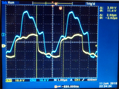
Starting CCW pulse signals, represented by blue on the oscilloscope, and returning bigger (gaining energy) from the 134 meters loop, represented by yellow on the below oscilloscope.

One important picture showing practically no anisotropy and no gain of energy of the same identical height ac pulses (Triangles on the left, indicate the zero point line of the two graphs respectively), departing and returning for a short loop of 0.7 meters, unlike the long 134 meters loop.

this time, as it has been described. This highlights our non-understanding of most properties of the fundamental Ether in the Universe.

What cannot be disputed at all is the fact that there is energy gained as creation of mass [11] , by both CCW and CW pulses. The returning long (134 m) pulses, as compared with the starting pulses, have an energy gain by 2 - 3 volts. Yes, you read well. The generator is giving first energy to overcome the resistive ≈12 ohm load of the of 134 m loop, but some, energy (not workless, as it happens with ac capacitors, for example, in ac circuits) is returned back to the source―generator, as an extra free present, as it happens to the famous “ball bearing motor” [12] . The wrong understanding of the nonexistence of the Ampere forces, controlled by their motion with respect to the Ether is not the only misconception of humans living on Earth. As we explained the Earth’s frame is considered inertial but this is wrong, due to the centripetal acceleration of its undisputed self-rotation. Also the Earth’s frame, because of the Earth’s rotation, is anisotropic. We have demonstrated and explained an anisotropy for long loop CCW and CW velocities, and anisotropic CW and CCW self-generating energy. Also, long loop CCW and CW velocities should cause the known slowing down of Earth’s rotation, known from 8 to 24 hours, and possibly also slow down other motions of Earth in the Universe just like friction. Thus humanity, ignoring the properties of the fundamental Ether in the Universe, has a lot more to learn yet in Physical science to reach the level of extra-terrestrials who can travel easily in the Universe.

Anyone is welcomed and invited to come and to be our guest and watch our above claims with his own eyes until he leaves 100% satisfied.

Cite this paper

Pappas, P.T., Jones, B.I., Pappas, T.P. and Pappas, L.P. (2018) Earth’s Serious Anisotropy, Non-Inertiality, Ether, Gain of Free Energy, Revealed, Part 2. Journal of Applied Mathematics and Physics, 6, 1332-1345. https://doi.org/10.4236/jamp.2018.66112

References

- 1. Pappas, P.T., Pappas, T.P and Pappas, L.P. (2017) Part 1 of This Present Paper. Important Discovery of Preferred Velocity of 30000 ± 425 M/S of the Solar Motion of the Earth, Part 1. Journal of Physical Mathematics, 8, 213.
- 2. Pappas, P.T. For the Raw Data of Measurements. http://www.panospappas.gr/
- 3. Net Charge of the Surface of the Earth. For Example, Physics Forums.https://www.physicsforums.com/threads/net-charge-of-the-surface-of-the-earth.771471/
- 4. Pappas, P.T. (2014) Ampere’s Force Law, Ampere Electrodynamics, Proof and Prediction of Empirical Faraday Induction. Physics Essays, 27, 570-579.
- 5. Earth Science. https://earthscience.stackexchange.com/questions/9907/how-long-does-a-magnetic-pole-reversal-take-to-complete
- 6. For Example Magnetic Reversal of the Poles of the Sun, NASA Report. https://www.nasa.gov/content/goddard/the-suns-magnetic-field-is-about-to-flip/ http://www.thesuntoday.org/solar-facts/suns-magnetic-poles-flipped-solar-max-is-here/ https://en.wikipedia.org/wiki/Geomagnetic_reversal
- 7. Pappas, P.T. (1995) Pappas Papimi.
- 8. Comet Tail Repelled Away from the Sun. https://en.wikipedia.org/wiki/Comet_tail
- 9. Spherical Capacitor Formula. http://hyperphysics.phy-astr.gsu.edu/hbase/electric/capsph.html
- 10. Dasgupta, A. (2018) Earth’s Centripetal Acceleration 0.0297m/s2. https://socratic.org/questions/what-is-the-magnitude-of-the-centripetal-acceleration-of-an-object-on-earth-s-eq
- 11. Theoharis, P.P. (2017) Mass Creation. Physical Science International Journal.
- 12. Pappas, P.T., Papps, T.P. and Pappas, L.P. (2018) Ball Bearing Motor. Journal of Applied Mathematics and Physics, 6.