Theoretical Economics Letters
Vol.2 No.5(2012), Article ID:25815,8 pages DOI:10.4236/tel.2012.25092
Estimating the Experience-Weighted Attractions for the Migration-Emission Game*
Center for Environmental Innovation Design for Sustainability, Osaka University, Osaka, Japan
Email: uwasu@ceids.osaka-u.ac.jp
Received July 5, 2012; revised August 7, 2012; accepted September 10, 2012
Keywords: Learning; Economic Experiments; Equilibrium Strategy
ABSTRACT
Players are unlikely to immediately play equilibrium strategies in complicated games or in games in which they do not have much experience playing. In these cases, players will need to learn to play equilibrium strategies. In laboratory experiments, subjects show systematic patterns of learning during a game. In psychological and economic models of learning, players tend to play a strategy more if it has been successful in the past (reinforcement learning) or that would have given higher payoffs given the strategies of other players (belief learning). This paper uses experimental data from the four sessions of a pilot experiment of a three-stage emission game to estimate parameters of experienceweighted-attraction (EWA) learning, which is a hybrid of reinforcement and belief learning models. In this estimation, we transform the strategy space for the three-stage game extensive form game to a normal form game. This paper also considers asymmetric information across players in estimating EWA parameters. In three of the four sessions, estimated parameters are consistent with reinforcement learning, which means that players tend to choose to strategies looking at past strategies that are more successful than the others. In the other session, estimated parameters are consistent with belief learning, which means that players consider forgone payoffs to update their beliefs that determine the probability of strategy choice.
1. Introduction
Game theory has made inroads in virtually all fields in economics and other social sciences. The equilibrium concepts in game theory are internally consistent, generating a clear prediction of how players should play in non-cooperative games. Empirical evidence, on the other hand, suggests people do not behave as game theory predicts even in simple games. Rather, it shows that people learn through a game, and typically they play an equilibrium strategy only as the game proceeds. How strategies evolve and how an equilibrium arises is of great interest. An equilibrium analysis approach, however, cannot show how equilibrium arises.
Development of theories of equilibrium dynamics arose to explain how players might arrive at equilibrium. In biology, evolutionary theory uses the idea of natural selection in which types with higher payoffs than average expand their share of the population. In economics, Cournot suggested simple dynamics more than a century ago in which players make a decision based on a best response to the previous round of play. Neither evolutionary nor Cournot theories fully incorporate learning. Evolutionary theory has no consideration of learning; equilibrium strategy is automatically determined by the initial share of strategies. Cournot dynamics are an extreme case of learning patterns and too simple to explore the players’ behavior. For example, Cournot dynamics counts only the most recent observations but it is possible that more previous observations also influence strategy choices.
While evidence of learning from laboratory experiments has been increasing, more detailed learning models have also been developed. These models have parameters that can be estimated using data from laboratory experiments. Two major learning models include reinforcement learning and belief learning. Reinforcement learning assumes that players tend to choose strategies that generated high payoffs in prior rounds. In reinforcement learning, attractions are used for numerical evaluations that determine the choice probability of strategies. Attractions are updated according to past strategy chosen by the player. Belief learning, on the other hand, assumes that players use forgone payoffs in the past to construct beliefs about what other players will do for future choices. Players update beliefs based on the past observations. Cournot dynamics is a special case of belief learning in which only the most recent observation is counted. Fictitious play is another type of belief learning model that counts all previous observations equally.
Several studies have compared these two learning models. The findings so far indicated that the performance of models depends on the games and no general conclusion has been drawn. Roth and Erev [1] showed that reinforcement learning performs better than belief learning in games with mixed strategy equilibrium (e.g., constant-sum games). On the other hand, Ho and Weigelt [2] showed that in games with multiple pure strategies (e.g., coordination games), a type of belief learning performed best.
Camerer and Ho [3] proposed EWA learning as a hybrid of reinforcement and belief learning. Like other learning models, in EWA, attractions determine the choice probability of strategies, and players update the attractions based on observations during the game. EWA learning has two key parameters. One parameter (δ in the model explained below) weighs between forgone payoffs and actually obtained payoffs in updating attractions and the other parameter (ϕ in the model explained below) discounts past attractions. With different values of these two parameters, EWA becomes either simple reinforcement learning or belief learning. EWA by construction contains both belief learning and reinforcement learning as special cases, so its fitness is at least as good as either of them. Put a different way, EWA always generates best fitness among the three learning models in terms loglikelihood statistics of estimates.
In this paper, I estimate parameters in EWA using experimental data obtained from the three stage emission game experiments conducted in Uwasu [4]. In this three stage emission game, players are initially assigned to one of the two equally-sized groups. In the first stage, players choose emission levels, “High” or “Low”. Emissions are thought of as a public bad so that they that negatively affects all players in the two groups. In the second stage, players who chose “Low” choose whether to punish those who chose “High” in the same group. In the third, players observe the average payoff of the other group and decide if they move to the other group. The evolutionary game model shows how cooperation emerges and how migration breaks down cooperation in the long term.
I deal with two features in estimating parameter values. First, a strategy space of an extensive form game for the EWA estimation is redefined as EWA deals with repeated games of normal form. The emission game used in the experiment consists of three stages including an activity stage, punishment stage, and migration stage. Since each stage has two discrete choices, the new strategy specification is made according to these strategy combinations. The choices made in the first two stages determine a player’s type; cooperators who chose “Low”, enforcers who chose “Low” and “Punishment”, and defectors who chose “High”. Further, each of the three types is differentiated by groups, which generates six strategies in each period. Thus, with this strategy transformation, players play a formal game with six strategies. Second, I deal with imperfect information across group members for the estimation. In the emission game, players can move across two groups while they share different information across groups. In EWA players use the average payoff of the other group and payoffs for each strategy in their group to decide whether to change groups. I construct information matrices for payoffs for the parameter estimations to take into account this asymmetric information across groups.
Data from four sessions in the three-stage emission game experiment are used to estimate EWA parameters. Predictive errors, differences between the number of actual choice of strategies and the predicted number are small across sessions. In C1 session (the session with 12 participants), the number of predicted strategy choices in the final round are the same as the actual number of strategy choices. In this session, two players moved from Group 2 to Group 1 and in the final period all players play “High” in the final period. The EWA learning produced the same strategy choices in the final period. In other words, EWA learning successfully shows how equilibrium strategy arises for this session.
The estimated parameters also show a consistent pattern of learning across sessions. Specifically, in three of the four sessions, players appear to follow reinforce learning, which means that players tend to choose strategies that are more successful than others. In one session, the estimated parameters suggest the belief learning, which indicates that players see payoffs from forgone strategies. The estimated initial attractions are also consistent with the game structure of the experiment. Strategies that involve punishment and migration have smaller value of initial attractions than other strategies. Similarly, attractions of enforcers in the group with a severer punishment rule are higher than those in the group with a soft punishment rule.
Next section explains EWA learning in details. Section 3 shows estimation strategies. Section 4 presents and discusses the results. Section 5 concludes the paper.
2. EWA Learning
Consider a normal form game with N players. Let Si be a set of pure strategies for player . The strategy space of the game is expressed as
  . There are J strategies so that let
  be a pure strategy for player i and
  be a strategy profile. The payoff for player i is given by
 . Assume that this game is finitely repeated for
  periods. Let
  denote a strategy chosen by player i in period t, and let
  denote player i’s payoff in period t.
EWA learning has two updated variables, attractions  and experience weights
  with given initial values of
  and
and  where the superscript j denotes a strategy and the subscript i denotes a player. An attraction determines the probabilities of strategy j being chosen at period t by player i. Each player has an attraction for each strategy and these are updated at the end of the period. Initial attractions,
  are estimated using data from laboratory experiment. The experience weight,
  can be thought of as a players experience that determines the speed of updating for attractions and an identical experience weight
  is given to attractions for all strategies. The initial experience weights are usually assumed to be identical across players with a value of
  for all i. This assumption has no substantial effects on the learning process (Camerer 2003).
An experience weight is updated according to
 (1)
(1)
where  is a depreciation rate of past experience and
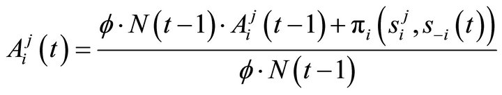
  is a parameter that determines the updateing speed of an experience weight. An attraction for strategy j for player i is updated according to (for t > 1)
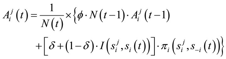 (2)
(2)
where  is an indicator
  if
if , and
, and  otherwise; and
  is called an imagination weight parameter.
Each parameter plays an important role. The parameter δ weighs the consideration of forgone payoffs (strategies that were not chosen in the past). The parameters ϕ discounts previous attractions. To make interpretation clear, it is useful to think special cases. When  and
and  with
with , the attraction updating rule becomes
 (3)
(3)
which is the reinforcement learning because attractions of the strategies that have been successful increase more quickly and forgone payoffs are ignored. On the other hand, when  and
and , the updating rule becomes
 (4)
(4)
which is the belief based model in the sense that strategies that were not chosen and a strategy that was chosen are equally considered in determining the future strategy choice.
Attractions are mapped into a probability distribution function that tells a probability of strategy j being chosen in a period t by player i (so that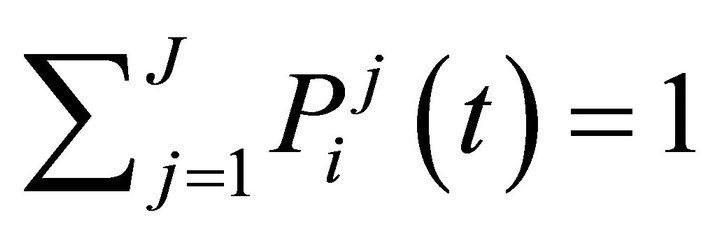 ). Typically, the logit form is used:
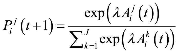 (5)
(5)
where λ is a payoff sensitivity parameter. The log-likelihood function is then written as
 (6)
(6)
3. The Game Structure and Estimation Strategy
3.1. The Game Structure
The game structure in this experiment is a three stage emission game with N players. There are two groups that initially have equal population size before the game starts. The three stage game with group division proceeds as follows.
Stage 1: Players get to see their earnings, the average earnings of their group, and the average earnings of the other group for the first two stages of the experiment in the previous round. Then, players choose whether to change groups. Changing groups is costly.
Stage 2: Players simultaneously choose emission levels, “High” or “Low”. The emission game is global pollution so that emissions negatively affect all the players in two groups.
Stage 3: Players observe actions in their group at the second stage. Players who chose “Low Activity” choose whether to punish those who chose “High Activity” in his group. Choosing punishment is costly and the two groups have different punishment cost structure: the punishment in one group is more severe to those who chose “High” than in the other.
What is an equilibrium strategy of this stage game? Note that Nash equilibrium of one shot emission game is “High” for all players. Thus, backward induction suggests that {“High”, “Not Punish”, “Not Move”} is a sub-game perfect equilibrium for the (one-period) three stage game. In a finitely repeated game of this three stage game, again backward induction suggests {“High”, “Not Punish”, “Not Move”} for all players in all periods is a subgame perfect equilibrium [4].
I used data from four experimental sessions for the estimation. These four sessions are different in several points. First, subjects’ background is different across sessions. In three of the four sessions, most subjects were from the Applied Economics and Economics Undergraduate Programs (econ), and in one session, subjects were from the Conservation Biology Graduate Program (cons bio). Second, in three of the four sessions, subjects got paid for the participation but in the other session subjects did not get paid. Third, these sessions are different in that subjects know each other in the experiment. In two sessions, subjects were recruited from several classes so that they were supposed to be strangers each other. But in the other two sessions, subjects were recruited from one class, so they might know each other. Finally, the number of rounds and players differ across sessions. Table 1 summarizes this information.
3.2. Estimation Strategy
The data used in the estimation are from the three-stage emission game experiment. The game in the experimental sessions is extensive form game. Because the EWA learning assumes a normal form game, the game needs to be redefined as a normal form game. Given the three stage with discrete choices, six combinations of players’ type can be constructed, as in Table 2.
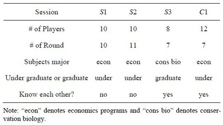
Table 1. Experimental Information.
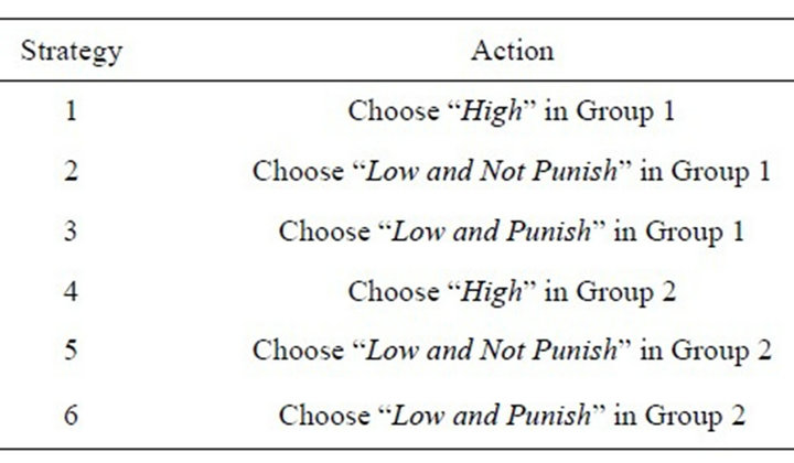
Table 2. Re-defined action space.
The definition of this strategy specification is similar to the concepts of “players’ type” in the evolutionary game model. Now, I show the estimation strategy.
• Step 1 Construct two information matrices using the experimental data: Let I be a  indicator matrix expressed as:
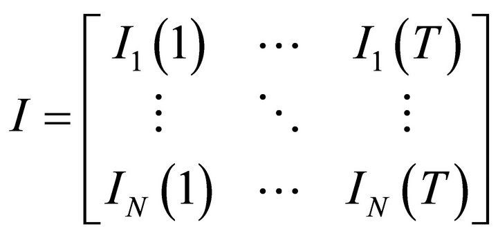 (7)
(7)
where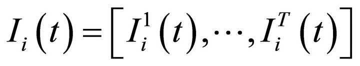 ’ is a 6 × 1 vector in which
  if
if and
and , otherwise.
Let Π is a  payoff matrix expressed as:
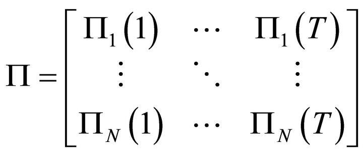 (8)
(8)
where ’ is a
  vector with
 .
.
Note that, in the experiment, players had six strategies; . If a player chose a strategy from
 (1,or 2,or 3) in period t-1, choosing a strategy from
  in period t requires him to move from Group 2 to Group 1 (or Group 1 to Group 2), which involves a moving cost. The moving cost is taken into account in constructing the payoff matrix for the parameter estimation. For example, if he chose Strategy 6 while he had chosen Strategy 1 in the previous period, he is supposed to move from Group 1 to Group 2 so that his payoff from choosing Strategy 6 is reduced by the moving cost.
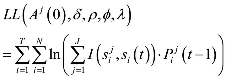
• Step 2 Write the log-likelihood function: Because the conditional logit function is a non-linear model, the estimation is done by a maximum likelihood method. The full log-likelihood function for our case can be then written as
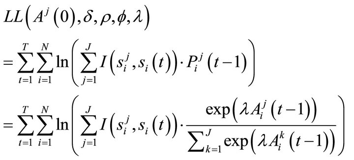 (9)
(9)
where λ is called a payoff sensitivity parameter.
The practical difficulty in estimation is that the arguments of the probability function are a non-linear functions of parameters. Moreover, the information used in the calculation of attractions varies over periods because it depends on the history of strategies. (For simplicity, the superscript j and the subscript i are omitted hereafter.) For example,  uses only
  and
and , but
, but  uses
uses  and
and  for all
 .
.
However, note the attraction updating Equation (2) is expanded to:
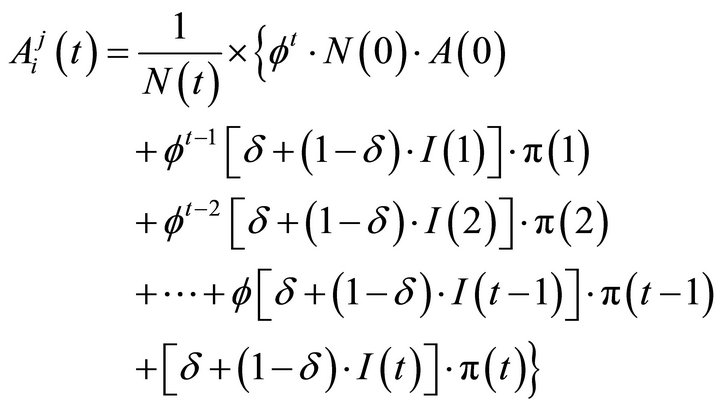
where  is a
is a  vector,
  is a scalar,
  and
and  are
are  vectors. (Those are from columns in the matrices I and Π, respectively: e.g.,
  is the first column of I). Furthermore, Camerer [5] states that the initial value of N has little effect on the process of learning, so
 . Having
  substantially simplifies the evolution of N:
 (11)
(11)
is here used. Using the Equations (10) and (11), we can explicitly write the log-likelihood function in MATLAB programming codes.
• Step 3 Maximize the likelihood function in MATLAB: Once a log-likelihood function is defined, it is maximized with respect to the parameters subject to ,
, by using a Newton method.
I assume that initial attractions are identical among initial group members, but they can be different across groups. Because I have two groups in all the experimental sessions, there are twelve initial attractions.
Finally, recall that attractions are mapped into a probability function to determine the probability of a strategy chosen. In order to have the sum of the probabilities be one, I fix one of the attractions for each group at zero. Thus there are ten initial attractions to be estimated. The total number of estimated parameters is therefore 15: 
 is
is  is
is  , δ, κ, ϕ, and, λ.
4. Results
Table 3 reports the estimation results for the four experimental sessions. The estimated learning parameters vary across sessions. However, Sessions 1, 2, and 3 have similar parameter values for δ and ϕ: δ are close to zero and ϕ are close to one. This combination of parameter values indicates reinforcement learning. Δ = 0 means that players do not consider forgone payoffs and ϕ = 1 means players equally weigh past experience. Meanwhile, players in S3 show a different learning pattern with δ = 0.62, and ϕ = 0. This indicates that the learning pattern is close to the belief learning with putting an equal consideration on what happened in the periods.
Note also that κ in the four sessions is close to one. Recall the parameter κ controls for the speed of growth of a particular attraction. The larger the κ is, the quicker the attraction grows. So, having κ = 1, players stick to playing the same strategy. This result makes sense because many players in the sessions tend to keep choosing the same strategy (i.e., “High”, “No Movement”, and “No Movement”) in the emission game.
The estimated parameters from the four sessions are plotted in an EWA parameter configuration box (Figure 1). This box clarifies the relationship between the values
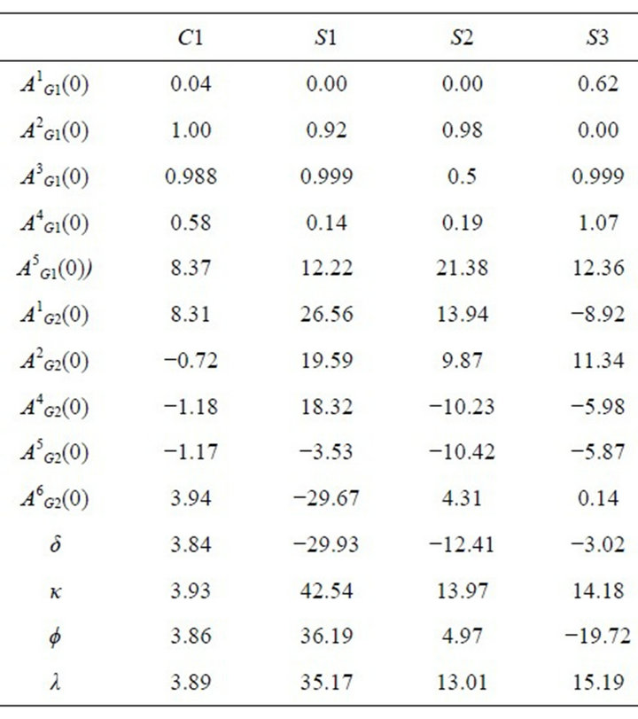
Table 3. Estimation results.
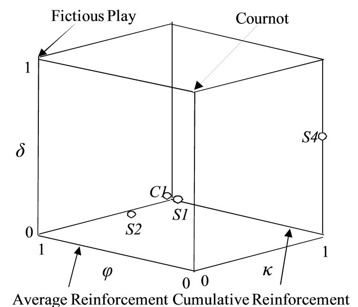
Figure 1. EWA parameter configuration box (Camerer [5]).
of each parameter and the corresponding learning patterns. For example, at the corner δ = 0 with κ = 0 or 1, this figure shows it is average reinforcement learning or cumulative learning. In average reinforcement learning, attractions do not cumulate but the rate of decay depends on the value of ϕ. In cumulative reinforcement learning, attractions cumulate so that players tend to stick to the same strategy. In this figure, it is clear that players in S1, S2, and C1 follow cumulative reinforcement (because of κ close to one) while those in S3 follow the belief learning.
Comparative studies of learning models have suggested that learning patterns differ across types of games [1,2,5]. However, we here observe different learning patterns in the same game. What possibly explains the difference in learning patterns across the sessions with the same game is the subjects’ characteristics. The subjects in S1, S2, and C1 were undergraduate students from intermediate economics classes. Subjects in S3 were graduate students majoring in conservation biology. Thus academic background and academic years are different in these two groups. Some studies show evidence that economics majors tend not to cooperate in the public goods game. Yet, these studies provide no evidence that the high likelihood of choosing defection emerged as a result of different learning pattern. A second possibility is the depth of understanding or educational levels. The EWA theory provides no clue about which learning is more advanced or requires more sophistication. There are other factors that affect learning patterns. For example, whether subjects know each other affects learning patterns. In fact, in S3, subjects knew each other, but it is true for C1 as well. Therefore, this stranger effect remains unclear.
We can see the estimated initial attractions reflect the observations in the experimental sessions. First, attracttions for strategies that require no migration seem to be higher than those for strategies that involve migration. (Higher values of attractions yield higher probabilities of choosing the strategy.) That is, for , attractions for
  are generally higher than those for
 . Likewise, for
 , attractions for
  are generally higher than those for
 . Second, comparing
  with
with , I show that Group 2 members are more likely to choose “Punish” than Group 1 members, which reflects the fact that Group 2 has a more severe punishment rule than Group 1. Uwasu [4] provided statistical evidence for this observation.
To see the overall fitness of EWA learning, I calculated predictive choice probabilities using the estimated parameter values. Figure 2 presents the predictive errors in choice probabilities for the four sessions. The predict-
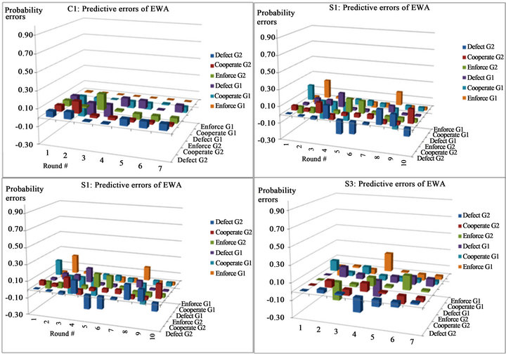
Figure 2. Predictive probabilities errors.
tive errors are calculated by taking the difference between actual choice probability and predictive probability. The largest errors of probabilities do not exceed 0.25 for one type in any period in the four sessions. In some rounds of sessions there are large predictive errors. The data from S1, S2, and S3 show that these large predictive errors are produced when there were sudden changes in strategy choices. For example, in S3 most players chose defection in Group 1 in the first three rounds, but in the fourth round, two enforcers suddenly emerged. The predictive error for this case was 0.22. Similar patterns are seen in the middle rounds of S1 and S2, too. Nevertheless, the large predictive errors shrink within two rounds of the game, which implies the reflection of attraction updating in the EWA learning.
Among the four sessions, EWA best fits the actual choices in C1 with the smallest predictive errors. I calculated the number of strategy choices using the predicted probability. Figure 3 shows the actual and predictive numbers of strategy choices for the class session as an example. In the final round, three of the three subjects in Group 1 and seven of the seven subjects in Group 2 chose “High” (Defector). And the predictive number of choices is exactly the same in the final round as the actual number. This is exactly the stable equilibrium in the context of evolutionary theory. In other words, EWA was able to show how equilibrium strategy arises in an observation at the laboratory level.
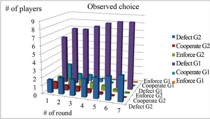 (a)
(a)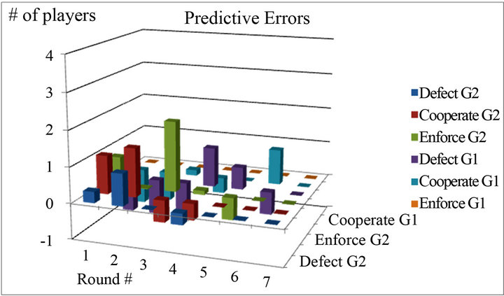 (b)
(b)
Figure 3. Actual vs. predictive numbers of strategy choices in C1.
5. Concluding Remarks
This paper estimated parameters in EWA learning using data from the three-stage emission game with punishment and endogenous grouping mechanism. The Maximum-likelihood estimation results showed a consistent pattern of learning across experimental sessions. In three of the four sessions, players are following reinforcement learning while one shows a type of belief learning. The EWA generated good fit to the real data and the predictive errors were small in most sessions. In one session, EWA produced stable equilibrium prediction. In general, EWA generated much better prediction of strategy choices than the evolutionary game models. Note that the evolutionary game model has no parameter that explains different learning patterns. For example, as explained in Uwasu [4], the evolutionary game model cannot explain a cyclical patter between choosing “High” and “Low” as in S1, EWA predicted more or less this choice pattern. In addition, the speed of learning in the evolutionary game model is very slow while players in the experiment use more information and thus learn more quickly. Finally, the results indeed had significant implications because even the seemingly identical equilibrium result is achieved through different paths. In particular, the estimation results suggest that the learning patterns are associated with players’ characteristics. The sessions with undergraduate economics majors showed reinforcement learning while a session with graduate conservation biology majors showed reinforcement learning. Experimental literature has examined how characteristics of players and groups such as gender, academic background, or knowing each other affect the provision of public goods [6,7]. Yet, to the best of my knowledge, no one has examined the question of how characteristics of players and groups such as gender, academic background, whether players know each other, affects learning behavior in games.
6. Acknowledgements
Part of this research was funded by Grant-in-Aid for Young Scientists (B) (2008-2009), the Ministry of Education, Culture, Sports, Science and Technology, Japan.
REFERENCES
- A. E. Roth and E. Ido, “Learning in Extensive Form Games: Experimental Data and Simple Dynamic Modelsin the Intermediate Term,” Games and Economic Behavior, Vol. 8, No. 1, 1995, pp. 164-212. doi:10.1016/S0899-8256(05)80020-X
- T. H. Ho and K. Weigelt, “Task Complexity, Equilibrium Selection, and Learning: An Experimental Study,” Management Science, Vol. 42, No. 5, 1996, pp. 659-679. doi:10.1287/mnsc.42.5.659
- C. Camerer and T. H. Ho, “Experienced-Weighted Attraction Learning in Normal Form Games,” Econometrica, Vol. 67, No. 4, 1999, pp. 827-874. doi:10.1111/1468-0262.00054
- M. Uwasu, “Essays on Environmental Cooperation,” Dissertation Thesis, University of Minnesota, Minnesota, 2008.
- C. Camerer, “Behavioral Game Theory: Experiments in Strategic Interaction,” Princeton University Press, Princeton, 2003.
- R. M. Isaac, K. McCue and C. Plott, “Public Goods Provision in an Experimental Environment,” Journal of Public Economics, Vol. 26, No. 1, 1985, pp. 51-74. doi:10.1016/0047-2727(85)90038-6
- J. Brown-Kruse and D. Hummels, “Gender Effects in Laboratory Public Goods Contribution: Do Individuals Put Their Money Where Their Mouth Is?” Journal of Economic Behavior and Organization, Vol. 22, No. 3, 1993, pp. 255-267. doi:10.1016/0167-2681(93)90001-6
NOTES
*This paper is based on Chapter 4 of the author’s dissertation that was submitted to University of Minnesota. I would like to express my appreciation to Stephen Polasky and Terrance Hurley for their valuable comments. All remaining errors are mine.