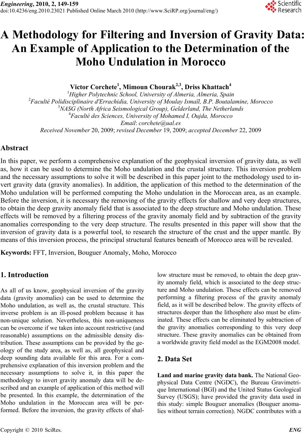Engineering, 2010, 2, 149-159
doi:10.4236/eng.2010.23021 lished Online March 2010 (http://www.SciRP.org/journal/eng/)
Pub
A Methodology for Filtering and Inversion of Gravity Data:
An Example of Application to the Determination of the
Moho Undulation in Morocco
Victor Corchete1, Mimoun Chourak2,3, Driss Khattach4
1Higher Polytechnic School, University of Almeria, Almeria, Spain
2Faculté Polidisciplinaire d'Errachidia, University of Moulay Ismaïl, B.P. Boutalamine, Morocco
3NASG (North Africa Seismological Group), Gelderland, The Netherlands
4Faculté des Sciences, University of Mohamed I, Oujda, Morocco
Received November 20, 2009; revised December 19, 2009; accepted December 22, 2009
Abstract
In this paper, we perform a comprehensive explanation of the geophysical inversion of gravity data, as well
as, how it can be used to determine the Moho undulation and the crustal structure. This inversion problem
and the necessary assumptions to solve it will be described in this paper joint to the methodology used to in-
vert gravity data (gravity anomalies). In addition, the application of this method to the determination of the
Moho undulation will be performed computing the Moho undulation in the Moroccan area, as an example.
Before the inversion, it is necessary the removing of the gravity effects for shallow and very deep structures,
to obtain the deep gravity anomaly field that is associated to the deep structure and Moho undulation. These
effects will be removed by a filtering process of the gravity anomaly field and by subtraction of the gravity
anomalies corresponding to the very deep structure. The results presented in this paper will show that the
inversion of gravity data is a powerful tool, to research the structure of the crust and the upper mantle. By
means of this inversion process, the principal structural features beneath of Morocco area will be revealed.
Keywords: FFT, Inversion, Bouguer Anomaly, Moho, Morocco
1. Introduction
As all of us know, geophysical inversion of the gravity
data (gravity anomalies) can be used to determine the
Moho undulation, as well as, the crustal structure. This
inverse problem is an ill-posed problem because it has
non-unique solution. Nevertheless, this non-uniqueness
can be overcome if we taken into account restrictive (and
reasonable) assumptions on the admissible density dis-
tribution. These assumptions can be provided by the ge-
ology of the study area, as well as, all geophysical and
deep sounding data available for this area. For a com-
prehensive explanation of this inversion problem and the
necessary assumptions to solve it, in this paper the
methodology to invert gravity anomaly data will be de-
scribed and an example of application of this method will
be presented. In this example, the determination of the
Moho undulation in the Moroccan area will be per-
formed. Before the inversion, the gravity effects of shal-
low structure must be removed, to obtain the deep grav-
ity anomaly field, which is associated to the deep struc-
ture and Moho undulation. These effects can be removed
performing a filtering process of the gravity anomaly
field, as it will be described below. The gravity effects of
structures deeper than the lithosphere also must be elim-
inated. These effects can be eliminated by subtraction of
the gravity anomalies corresponding to this very deep
structure. These gravity anomalies can be obtained from
a worldwide gravity field model as the EGM2008 model.
2. Data Set
Land and marine gravity data bank. The National Geo-
physical Data Centre (NGDC), the Bureau Gravimetri-
que International (BGI) and the United Status Geological
Survey (USGS); have provided the gravity data used in
this study: simple Bouguer anomalies (Bouguer anoma-
lies without terrain correction). NGDC contributes with a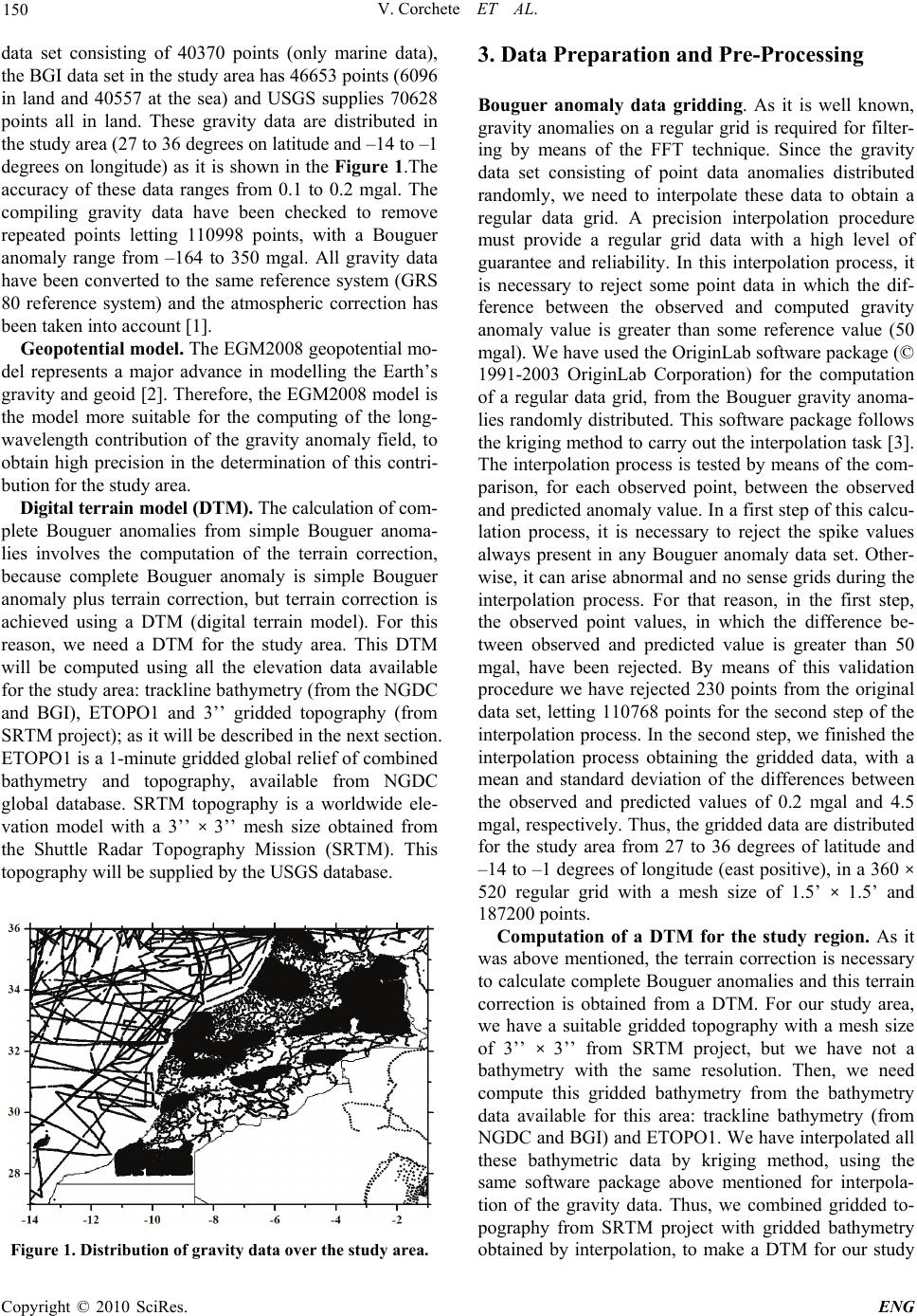

V. Corchete ET AL. 150
data set consisting of 40370 points (only marine data),
the BGI data set in the study area has 46653 points (6096
in land and 40557 at the sea) and USGS supplies 70628
points all in land. These gravity data are distributed in
the study area (27 to 36 degrees on latitude and –14 to –1
degrees on longitude) as it is shown in the Figure 1.The
accuracy of these data ranges from 0.1 to 0.2 mgal. The
compiling gravity data have been checked to remove
repeated points letting 110998 points, with a Bouguer
anomaly range from –164 to 350 mgal. All gravity data
have been converted to the same reference system (GRS
80 reference system) and the atmospheric correction has
been taken into account [1].
Geopotential model. The EGM2008 geopotential mo-
del represents a major advance in modelling the Earth’s
gravity and geoid [2]. Therefore, the EGM2008 model is
the model more suitable for the computing of the long-
wavelength contribution of the gravity anomaly field, to
obtain high precision in the determination of this contri-
bution for the study area.
Digital terrain model (DTM). The calculation of com-
plete Bouguer anomalies from simple Bouguer anoma-
lies involves the computation of the terrain correction,
because complete Bouguer anomaly is simple Bouguer
anomaly plus terrain correction, but terrain correction is
achieved using a DTM (digital terrain model). For this
reason, we need a DTM for the study area. This DTM
will be computed using all the elevation data available
for the study area: trackline bathymetry (from the NGDC
and BGI), ETOPO1 and 3’’ gridded topography (from
SRTM project); as it will be described in the next section.
ETOPO1 is a 1-minute gridded global relief of combined
bathymetry and topography, available from NGDC
global database. SRTM topography is a worldwide ele-
vation model with a 3’’ × 3’’ mesh size obtained from
the Shuttle Radar Topography Mission (SRTM). This
topography will be supplied by the USGS database.
Figure 1. Distribution of gravity data over the study area.
3. Data Preparation and Pre-Processing
Bouguer anomaly data gridding. As it is well known,
gravity anomalies on a regular grid is required for filter-
ing by means of the FFT technique. Since the gravity
data set consisting of point data anomalies distributed
randomly, we need to interpolate these data to obtain a
regular data grid. A precision interpolation procedure
must provide a regular grid data with a high level of
guarantee and reliability. In this interpolation process, it
is necessary to reject some point data in which the dif-
ference between the observed and computed gravity
anomaly value is greater than some reference value (50
mgal). We have used the OriginLab software package (©
1991-2003 OriginLab Corporation) for the computation
of a regular data grid, from the Bouguer gravity anoma-
lies randomly distributed. This software package follows
the kriging method to carry out the interpolation task [3].
The interpolation process is tested by means of the com-
parison, for each observed point, between the observed
and predicted anomaly value. In a first step of this calcu-
lation process, it is necessary to reject the spike values
always present in any Bouguer anomaly data set. Other-
wise, it can arise abnormal and no sense grids during the
interpolation process. For that reason, in the first step,
the observed point values, in which the difference be-
tween observed and predicted value is greater than 50
mgal, have been rejected. By means of this validation
procedure we have rejected 230 points from the original
data set, letting 110768 points for the second step of the
interpolation process. In the second step, we finished the
interpolation process obtaining the gridded data, with a
mean and standard deviation of the differences between
the observed and predicted values of 0.2 mgal and 4.5
mgal, respectively. Thus, the gridded data are distributed
for the study area from 27 to 36 degrees of latitude and
–14 to –1 degrees of longitude (east positive), in a 360 ×
520 regular grid with a mesh size of 1.5’ × 1.5’ and
187200 points.
Computation of a DTM for the study region. As it
was above mentioned, the terrain correction is necessary
to calculate complete Bouguer anomalies and this terrain
correction is obtained from a DTM. For our study area,
we have a suitable gridded topography with a mesh size
of 3’’ × 3’’ from SRTM project, but we have not a
bathymetry with the same resolution. Then, we need
compute this gridded bathymetry from the bathymetry
data available for this area: trackline bathymetry (from
NGDC and BGI) and ETOPO1. We have interpolated all
these bathymetric data by kriging method, using the
same software package above mentioned for interpola-
tion of the gravity data. Thus, we combined gridded to-
pography from SRTM project with gridded bathymetry
obtained by interpolation, to make a DTM for our study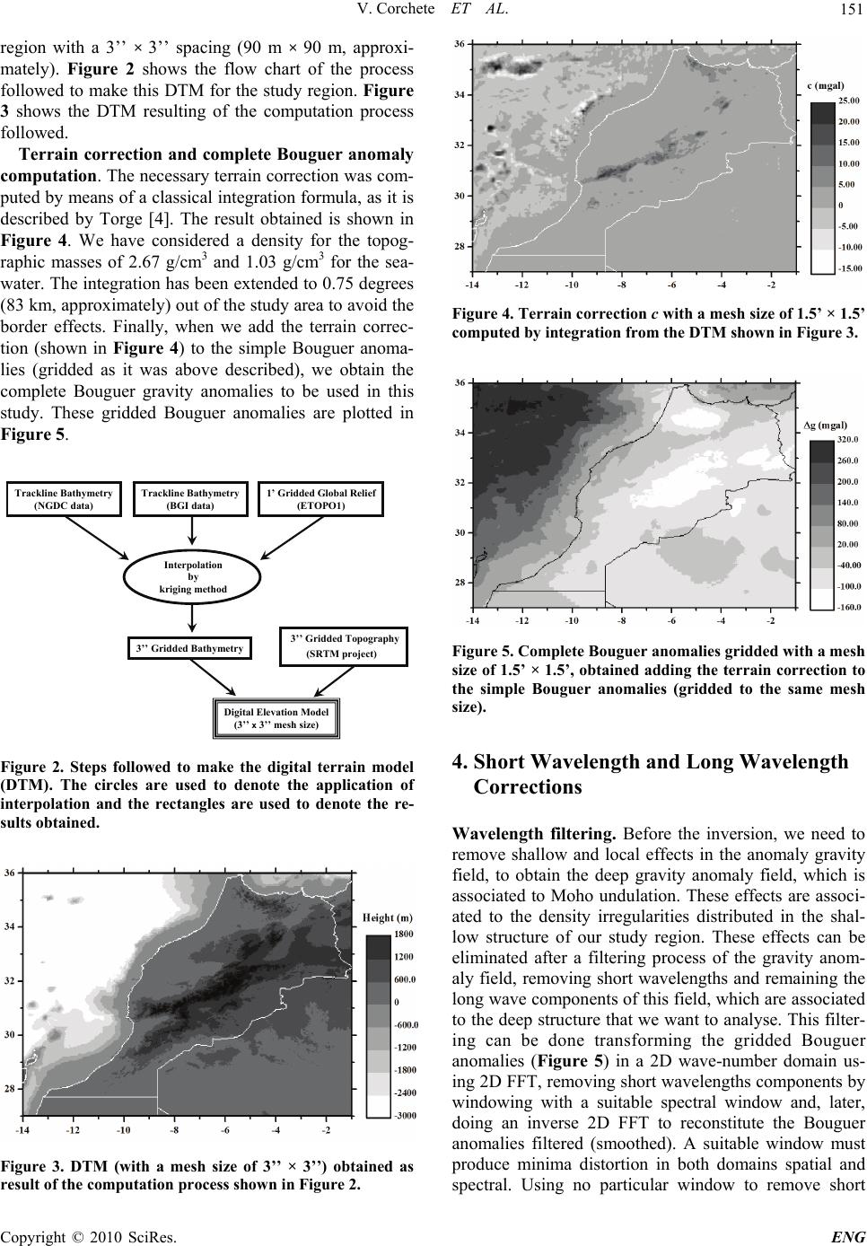

V. Corchete ET AL. 151
region with a 3’’ × 3’’ spacing (90 m × 90 m, approxi-
mately). Figure 2 shows the flow chart of the process
followed to make this DTM for the study region. Figure
3 shows the DTM resulting of the computation process
followed.
Terrain correction and complete Bouguer anomaly
computation. The necessary terrain correction was com-
puted by means of a classical integration formula, as it is
described by Torge [4]. The result obtained is shown in
Figure 4. We have considered a density for the topog-
raphic masses of 2.67 g/cm3 and 1.03 g/cm3 for the sea-
water. The integration has been extended to 0.75 degrees
(83 km, approximately) out of the study area to avoid the
border effects. Finally, when we add the terrain correc-
tion (shown in Figure 4) to the simple Bouguer anoma-
lies (gridded as it was above described), we obtain the
complete Bouguer gravity anomalies to be used in this
study. These gridded Bouguer anomalies are plotted in
Figure 5.
3’’ Gridded Bathymetry
3’’ Gridded Topography
(SRTM project)
Trackline Bathymetry
(NGDC data)
Trackline Bathymetry
(BGI data)
1’ Gridded Global Relief
(ETOPO1)
Interpolation
by
kriging method
Digital Elevation Model
(3’’
x 3’’ mesh size)
Figure 2. Steps followed to make the digital terrain model
(DTM). The circles are used to denote the application of
interpolation and the rectangles are used to denote the re-
sults obtained.
Figure 3. DTM (with a mesh size of 3’’ × 3’’) obtained as
result of the computation process shown in Figure 2.
Figure 4. Terrain correction c with a mesh size of 1.5’ × 1.5’
computed by integration from the DTM shown in Figure 3.
Figure 5. Complete Bouguer anomalies gridded with a mesh
size of 1.5’ × 1.5’, obtained adding the terrain correction to
the simple Bouguer anomalies (gridded to the same mesh
size).
4. Short Wavelength and Long Wavelength
Corrections
Wavelength filtering. Before the inversion, we need to
remove shallow and local effects in the anomaly gravity
field, to obtain the deep gravity anomaly field, which is
associated to Moho undulation. These effects are associ-
ated to the density irregularities distributed in the shal-
low structure of our study region. These effects can be
eliminated after a filtering process of the gravity anom-
aly field, removing short wavelengths and remaining the
long wave components of this field, which are associated
to the deep structure that we want to analyse. This filter-
ing can be done transforming the gridded Bouguer
anomalies (Figure 5) in a 2D wave-number domain us-
ing 2D FFT, removing short wavelengths components by
windowing with a suitable spectral window and, later,
doing an inverse 2D FFT to reconstitute the Bouguer
anomalies filtered (smoothed). A suitable window must
produce minima distortion in both domains spatial and
spectral. Using no particular window to remove short
C opyright © 2010 SciRes. ENG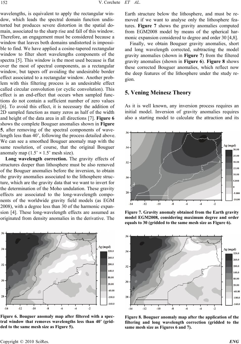

V. Corchete ET AL. 152
wavelengths, is equivalent to apply the rectangular win-
dow, which leads the spectral domain function undis-
torted but produces severe distortion in the spatial do-
main, associated to the sharp rise and fall of this window.
Therefore, an engagement must be considered because a
window that leaves both domains undistorted is impossi-
ble to find. We have applied a cosine-tapered rectangular
window to filter short wavelengths components of the
spectra [5]. This window is the most used because is flat
over the most of spectral components, as a rectangular
window, but tapers off avoiding the undesirable border
effect associated to a rectangular window. Another prob-
lem with this filtering process is an undesirable effect
called circular convolution (or cyclic convolution). This
effect is an end-effect that occurs when sampled func-
tions do not contain a sufficient number of zero values
[6]. To avoid this effect, it is necessary the addition of
2D sampled function as many zeros as half of the width
and height of the data area in all directions [7]. Figure 6
shows the complete Bouguer anomalies shown in Figure
5, after removing of the spectral components of wave-
length less than 40’, following the process detailed above.
We can see a smoothed Bouguer anomaly map with the
same resolution, of course, that the original Bouguer
anomaly map (1.5’ × 1.5’ mesh size).
Long wavelength correction. The gravity effects of
structures deeper than lithosphere must be also removed
of the Bouguer anomalies before the inversion, to obtain
the gravity anomalies associated to the lithosphere struc-
ture, which are the gravity data that we want to invert for
the determination of the Moho undulation. These gravity
effects are associated to the long-wavelength compo-
nents of the worldwide gravity field models (as EGM
2008), with a degree less than 30 of the harmonic expan-
sion [4]. These long-wavelength effects are assumed as
originated from density anomalies in the derivative. The
Figure 6. Bouguer anomaly map after filtered with a spec-
tral window that removes wavelengths less than 40’ (grid-
ded to the same mesh size as Figure 5).
Earth structure below the lithosphere, and must be re-
moved if we want to analyse only the lithosphere fea-
tures. Figure 7 shows the gravity anomalies computed
from EGM2008 model by means of the spherical har-
monic expansion considered to degree and order 30 [4,8].
Finally, we obtain Bouguer gravity anomalies, short
and long wavelength corrected, subtracting the model
gravity anomalies (shown in Figure 7) from the filtered
gravity anomalies (shown in Figure 6). Figure 8 shows
these corrected Bouguer anomalies, which reflect now
the deep features of the lithosphere under the study re-
gion.
5. Vening Meinesz Theory
As it is well known, any inversion process requires an
initial model. Inversion of gravity anomalies requires
also a starting model to calculate the attraction and its
Figure 7. Gravity anomaly obtained from the Earth gravity
model EGM2008, considering maximum degree and order
equals to 30 (gridded to the same mesh size as Figure 6).
Figure 8. Bouguer anomaly map after the application of the
filtering and long wavelength correction (gridded to the
same mesh size as Figures 6 and 7).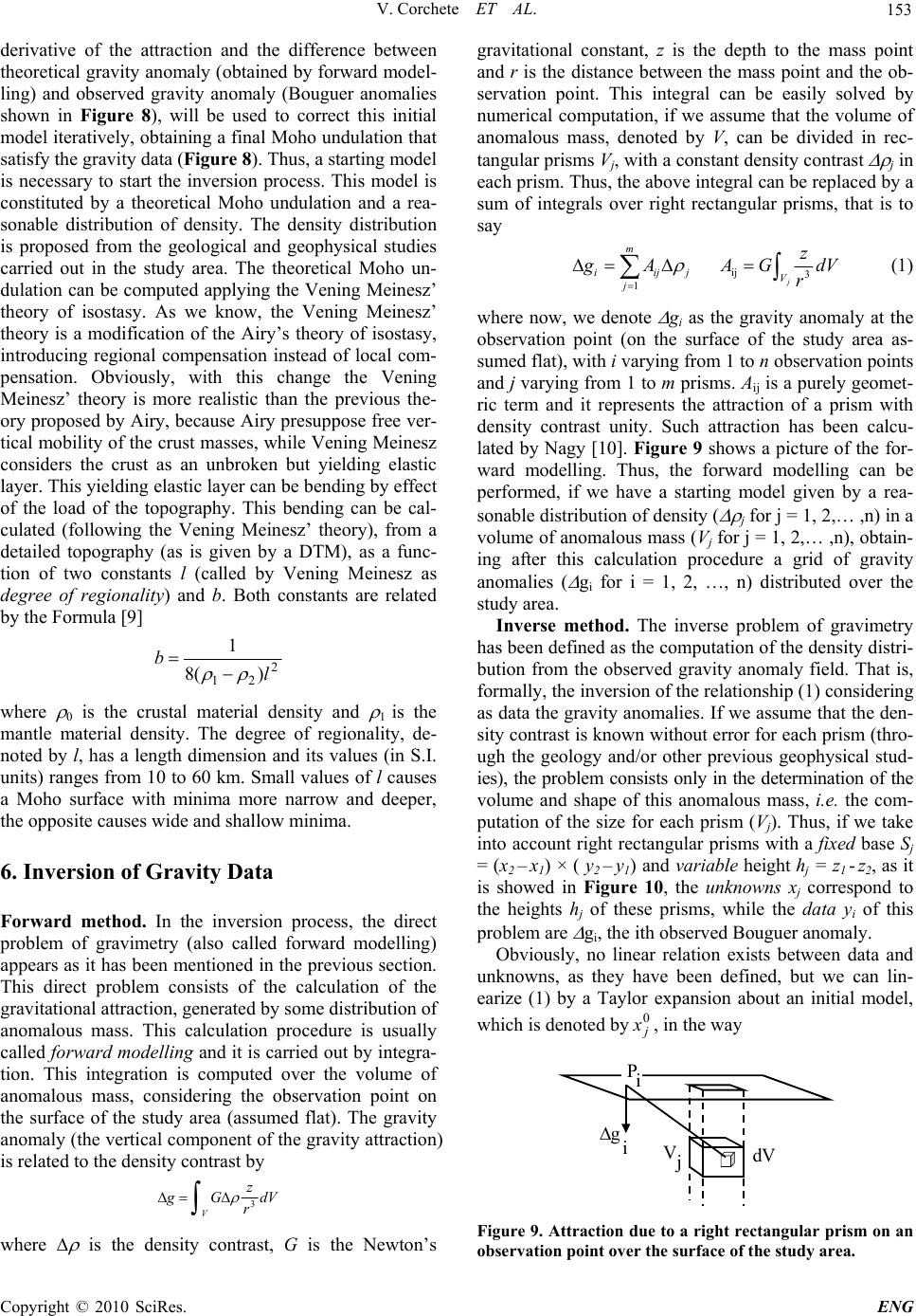

V. Corchete ET AL. 153
derivative of the attraction and the difference between
theoretical gravity anomaly (obtained by forward model-
ling) and observed gravity anomaly (Bouguer anomalies
shown in Figure 8), will be used to correct this initial
model iteratively, obtaining a final Moho undulation that
satisfy the gravity data (Figure 8). Thus, a starting model
is necessary to start the inversion process. This model is
constituted by a theoretical Moho undulation and a rea-
sonable distribution of density. The density distribution
is proposed from the geological and geophysical studies
carried out in the study area. The theoretical Moho un-
dulation can be computed applying the Vening Meinesz’
theory of isostasy. As we know, the Vening Meinesz’
theory is a modification of the Airy’s theory of isostasy,
introducing regional compensation instead of local com-
pensation. Obviously, with this change the Vening
Meinesz’ theory is more realistic than the previous the-
ory proposed by Airy, because Airy presuppose free ver-
tical mobility of the crust masses, while Vening Meinesz
considers the crust as an unbroken but yielding elastic
layer. This yielding elastic layer can be bending by effect
of the load of the topography. This bending can be cal-
culated (following the Vening Meinesz’ theory), from a
detailed topography (as is given by a DTM), as a func-
tion of two constants l (called by Vening Meinesz as
degree of regionality) and b. Both constants are related
by the Formula [9]
2
21 )(8
1
l
b
 

where 
0 is the crustal material density and

1 is the
mantle material density. The degree of regionality, de-
noted by l, has a length dimension and its values (in S.I.
units) ranges from 10 to 60 km. Small values of l causes
a Moho surface with minima more narrow and deeper,
the opposite causes wide and shallow minima.
6. Inversion of Gravity Data
Forward method. In the inversion process, the direct
problem of gravimetry (also called forward modelling)
appears as it has been mentioned in the previous section.
This direct problem consists of the calculation of the
gravitational attraction, generated by some distribution of
anomalous mass. This calculation procedure is usually
called forward modelling and it is carried out by integra-
tion. This integration is computed over the volume of
anomalous mass, considering the observation point on
the surface of the study area (assumed flat). The gravity
anomaly (the vertical component of the gravity attraction)
is related to the density contrast by
dV
r
z
Gg
V
3


where 
 is the density contrast, G is the Newton’s
gravitational constant, z is the depth to the mass point
and r is the distance between the mass point and the ob-
servation point. This integral can be easily solved by
numerical computation, if we assume that the volume of
anomalous mass, denoted by V, can be divided in rec-
tangular prisms Vj, with a constant density contrast

j in
each prism. Thus, the above integral can be replaced by a
sum of integrals over right rectangular prisms, that is to
say
ij 3
1
j
m
iijj V
j
z
g
AAG
r


 
dV (1)
where now, we denote
 gi as the gravity anomaly at the
observation point (on the surface of the study area as-
sumed flat), with i varying from 1 to n observation points
and j varying from 1 to m prisms. Aij is a purely geomet-
ric term and it represents the attraction of a prism with
density contrast unity. Such attraction has been calcu-
lated by Nagy [10]. Figure 9 shows a picture of the for-
ward modelling. Thus, the forward modelling can be
performed, if we have a starting model given by a rea-
sonable distribution of density (

j for j = 1, 2,… ,n) in a
volume of anomalous mass (Vj for j = 1, 2,… ,n), obtain-
ing after this calculation procedure a grid of gravity
anomalies (
 gi for i = 1, 2, …, n) distributed over the
study area.
Inverse method. The inverse problem of gravimetry
has been defined as the computation of the density distri-
bution from the observed gravity anomaly field. That is,
formally, the inversion of the relationship (1) considering
as data the gravity anomalies. If we assume that the den-
sity contrast is known without error for each prism (thro-
ugh the geology and/or other previous geophysical stud-
ies), the problem consists only in the determination of the
volume and shape of this anomalous mass, i.e. the com-
putation of the size for each prism (Vj). Thus, if we take
into account right rectangular prisms with a fixed base Sj
= (x2 – x1) × ( y2 – y1) and variable height hj = z1 - z2, as it
is showed in Figure 10, the unknowns xj correspond to
the heights hj of these prisms, while the da ta yi of this
problem are
 gi, the ith observed Bouguer anomaly.
Obviously, no linear relation exists between data and
unknowns, as they have been defined, but we can lin-
earize (1) by a Taylor expansion about an initial model,
which is denoted by, in the way
0
j
x
Pi
VjdV
gi
Figure 9. Attraction due to a right rectangular prism on an
observation point over the surface of the study area.
C opyright © 2010 SciRes. ENG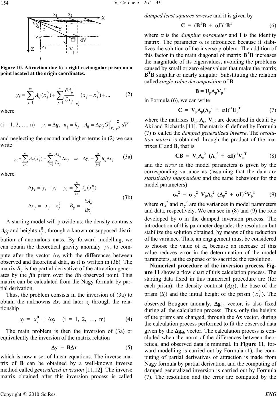

V. Corchete ET AL. 154
Vj
dV
r
X
Y
Zz
z
1
2
xx
12
yy
12
Figure 10. Attraction due to a right rectangular prism on a
point located at the origin coordinates.
...)()( 0
1
0
10



  
jj
x
m
jj
ij
j
m
j
iji xx
x
A
xAy
j
(2)
where
(i = 1, 2, …, n) jij 3 x
j
ii jj
V
z
yghAG d
r
  V
and neglecting the second and higher terms in (2) we can
write
j
m
j
ijj
m
jj
ij
j
m
j
iji xBx
x
A
xAy


   1
i
1
0
1
y )( (3a)
where
0
1
0
()
m
iiiiijj
j
ij
jjjij
j
yyyyAx
A
xxxB x

 

 


(3b)
A starting model will provide us: the density contrasts

j and heights; through a known or supposed distri-
bution of anomalous mass. By forward modelling, we
can obtain the theoretical gravity anomaly
0
j
x
i
y, to com-
pute after the vector yi with the differences between
observed and theoretical data, as it is written in (3b). The
matrix Bij is the partial derivative of the attraction gener-
ates by the jth prism over the ith observed point. This
matrix can be calculated from the Nagy formula by par-
tial derivation.
Thus, the problem consists in the inversion of (3a) to
obtain the unknowns  xj and later xj through the rela-
tionship
xj = + xj (j = 1, 2, …, m) (4)
0
j
x
The main problem is then the inversion of (3a) or
equivalently the inversion of the matrix relation
y = Bx (5)
which is now a set of linear equations. The inverse ma-
trix of B can be obtained by a well-known inverse
method called generalized inversion [11,12]. The inverse
matrix obtained after this inversion process is called
damped least squares inverse and it is given by
C = (BTB + I)-1BT (6)
where is the damping parameter and I is the identity
matrix. The parameter  is introduced because it stabi-
lizes the solution of the inverse problem. The addition of
this factor in the main diagonal of matrix BTB increases
the magnitude of its eigenvalues, avoiding the problems
caused by small or zero eigenvalues that make the matrix
BTB singular or nearly singular. Substituting the relation
called single value decomposition of B
B = UppVp
T
in Formula (6), we can write
C = Vpp(p
2 + I)-1Up T (7)
where the matrixes Up, p, Vp; are described in detail by
Aki and Richards [11]. The matrix C defined by Formula
(7) is called the damped generalized inverse. The resolu-
tion matrix is obtained through the product of the ma-
trixes C and B, that is
CB = Vpp
2 (p 2 + I)-1Vp T (8)
and the error in the model parameters is given by the
corresponding variance as (assuming that the data are
statistically independent and the same behaviour for the
model parameters)
x
2 =  y 2 V
pp
2 (p 2 + I)-2Vp T (9)
where  x
2 and  y 2 are the variances in model parameters
and data, respectively. We can see in (8) and (9) the role
developed by in the damped inversion process. The
introduction of this parameter degrades the resolution but
stabilize the solution obtained, by means of the reduction
of the variance. Thus, an engagement must be considered
to choose the value of , because an increase of this
value reduces error in the determination of the model
parameters, at the expense of to sacrifice the resolution.
Numerical procedure of the inversion process. Fig-
ure 11 shows a flow chart of this calculation process. The
starting data fixed in this numerical procedure are (for
each prism): the density contrast ( 
j), the base of the
prism (Sj) and the initial height of the prism (). The
observed Bouguer anomaly, gob vector, is also fixed
during all the calculation process. Thus, only the heights
of the prisms are changed, through the x vector, during
the calculation process performed to fit the observed data
given by the gob vector. The calculation process is con-
cluded when the norm of the differences between theo-
retical and observed data is minimal. In Figure 11, for-
ward modelling is carried out by Formula (1), the com-
puting of partial derivatives of attraction is made from
Nagy formula by partial derivation, and the computing of
damped generalized inversion is carried out by Formula
0
j
x
(7). The resolution and the error are computed by the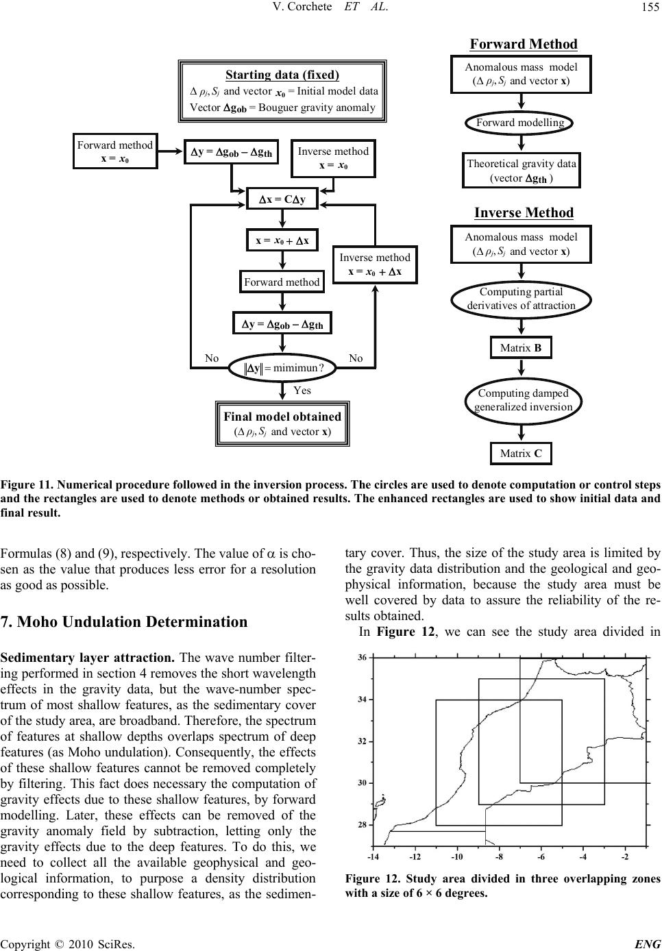

V. Corchete ET AL. 155
Starting data (fixed)

j
, S
j
and vector x
0
= Initial model data
Vector g
ob
= Bouguer gravity anomaly
y = g
ob
g
th
x = Cy
x = x
0
x
Forward method
y = g
ob
g
th
?mimimun

y
Yes
Final model obtained
(
j
, S
j
and vector x)
NoNo
Computing partial
derivatives of attraction
Matrix B
Computing damped
generalized inversion
Matrix C
Anomalous mass model
(
j
, S
j
and vector x)
Inverse Method
Forward modelling
Theoretical gravity data
(vector g
th
)
Anomalous mass model
(
j
, S
j
and vector x)
Forward Method
Inverse method
x = x
0
x
Inverse method
x = x
0
Forward method
x = x
0
ρ
j
, S
j
x
0
ρ
j
, S
j
x
0
x
0
x
0
x
0
ρ
j
, S
j
ρ
j
, S
j
Figure 11. Numerical procedure followed in the inversion process. The circles are used to denote computation or control steps
and the rectangles are used to denote methods or obtained results. The enhanced rectangles are used to show initial data and
final result.
Formulas (8) and (9), respectively. The value of  is cho-
sen as the value that produces less error for a resolution
as good as possible.
7. Moho Undulation Determination
Sedimentary layer attraction. The wave number filter-
ing performed in section 4 removes the short wavelength
effects in the gravity data, but the wave-number spec-
trum of most shallow features, as the sedimentary cover
of the study area, are broadband. Therefore, the spectrum
of features at shallow depths overlaps spectrum of deep
features (as Moho undulation). Consequently, the effects
of these shallow features cannot be removed completely
by filtering. This fact does necessary the computation of
gravity effects due to these shallow features, by forward
modelling. Later, these effects can be removed of the
gravity anomaly field by subtraction, letting only the
gravity effects due to the deep features. To do this, we
need to collect all the available geophysical and geo-
logical information, to purpose a density distribution
corresponding to these shallow features, as the sedimen-
tary cover. Thus, the size of the study area is limited by
the gravity data distribution and the geological and geo-
physical information, because the study area must be
well covered by data to assure the reliability of the re-
sults obtained.
In Figure 12, we can see the study area divided in
Figure 12. Study area divided in three overlapping zones
with a size of 6 × 6 degrees.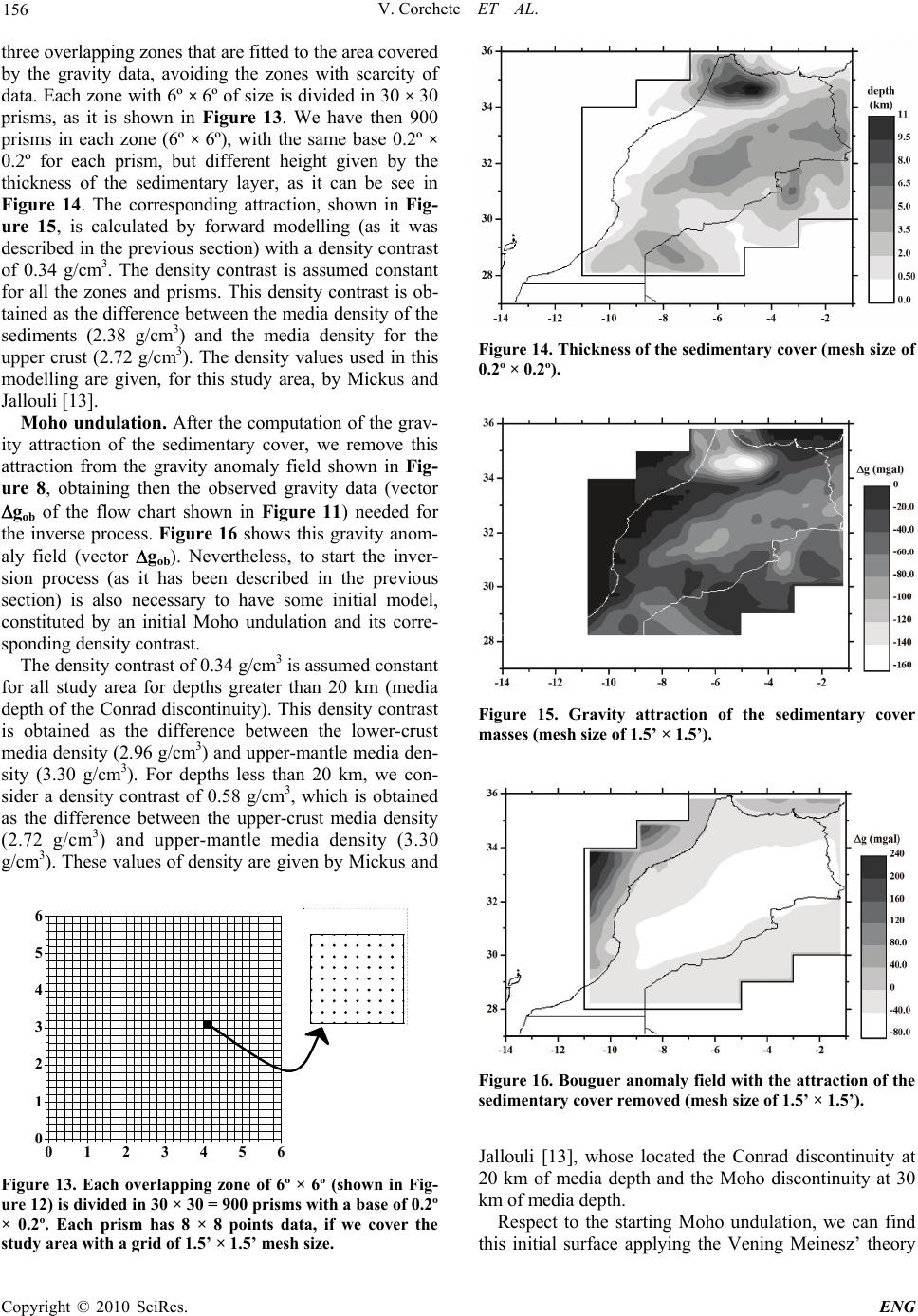

V. Corchete ET AL. 156
three overlapping zones that are fitted to the area covered
by the gravity data, avoiding the zones with scarcity of
data. Each zone with 6º × 6º of size is divided in 30 × 30
prisms, as it is shown in Figure 13. We have then 900
prisms in each zone (6º × 6º), with the same base 0.2º ×
0.2º for each prism, but different height given by the
thickness of the sedimentary layer, as it can be see in
Figure 14. The corresponding attraction, shown in Fig-
ure 15, is calculated by forward modelling (as it was
described in the previous section) with a density contrast
of 0.34 g/cm3. The density contrast is assumed constant
for all the zones and prisms. This density contrast is ob-
tained as the difference between the media density of the
sediments (2.38 g/cm3) and the media density for the
upper crust (2.72 g/cm3). The density values used in this
modelling are given, for this study area, by Mickus and
Jallouli [13].
Moho undulation. After the computation of the grav-
ity attraction of the sedimentary cover, we remove this
attraction from the gravity anomaly field shown in Fig-
ure 8, obtaining then the observed gravity data (vector
gob of the flow chart shown in Figure 11) needed for
the inverse process. Figure 16 shows this gravity anom-
aly field (vector gob). Nevertheless, to start the inver-
sion process (as it has been described in the previous
section) is also necessary to have some initial model,
constituted by an initial Moho undulation and its corre-
sponding density contrast.
The density contrast of 0.34 g/cm3 is assumed constant
for all study area for depths greater than 20 km (media
depth of the Conrad discontinuity). This density contrast
is obtained as the difference between the lower-crust
media density (2.96 g/cm3) and upper-mantle media den-
sity (3.30 g/cm3). For depths less than 20 km, we con-
sider a density contrast of 0.58 g/cm3, which is obtained
as the difference between the upper-crust media density
(2.72 g/cm3) and upper-mantle media density (3.30
g/cm3). These values of density are given by Mickus and
0123456
0
1
2
3
4
5
6
Figure 13. Each overlapping zone of 6º × 6º (shown in Fig-
ure 12) is divided in 30 × 30 = 900 prisms with a base of 0.2º
× 0.2º. Each prism has 8 × 8 points data, if we cover the
study area with a grid of 1.5’ × 1.5’ mesh size.
Figure 14. Thickness of the sedimentary cover (mesh size of
0.2º × 0.2º).

Figure 15. Gravity attraction of the sedimentary cover
masses (mesh size of 1.5’ × 1.5’).


Figure 16. Bouguer anomaly field with the attraction of the
sedimentary cover removed (mesh size of 1.5’ × 1.5’).

Jallouli [13], whose located the Conrad discontinuity at
20 km of media depth and the Moho discontinuity at 30
km of media depth.
Respect to the starting Moho undulation, we can find
this initial surface applying the Vening Meinesz’ theory

V. Corchete ET AL. 157
of isostasy, as it was described in section 5, considering a
suitable value for the degree of regionality. We take this
value as 26 km, because the Moho surface obtained for
this value gives, through forward modelling, a gravity
attraction field that is the most near to the observed grav-
ity filed (as it can be seen by comparison between Fig-
ures 16 and 18). Figure 17 shows this starting Moho
undulation obtained for the degree of regionality of 26
km. Figure 18 shows the theoretical gravity anomaly
obtained, by forward modelling, from this starting model.
Once the starting data of the inversion process have been
established, we can proceed to invert the gravity data as
it was described in the previous section, obtaining the
final Moho undulation shown in Figure 19. The errors in
the Moho depth are computed by Formula (9). These
errors raging between 0.02 and 0.7 km of standard devia-
tion, but the major part of them are around 0.5 km.
Figure 17. Moho depth predicted by Vening Meinesz’ the-
ory (mesh size of 0.2º × 0.2º).
8. Interpretation and Conclusions
The results presented in this paper show that the inver-
sion of gravity data is a powerful tool, to investigate the
structure of the crust and upper mantle. By means of this
technique are revealed the principal structural features
beneath of Morocco. Such features are the existence of
lateral and vertical heterogeneity in the study area, as it is
concluded when we see Figure 20, in which a general
picture of the lithospheric structure is shown from 0 to
50 km. In this Figure, several Moho profiles performed
in the study area show the different ways to make thin
the crust.
Figure 18. Theoretical Bouguer anomaly obtained by forward
modelling from the starting model (mesh size of 1.5’ × 1.5’).
Figure 19. Moho depth distribution after the inversion process (mesh size of 0.2º × 0.2º).

V. Corchete ET AL. 158
Moho Undulation Profiles
36
34
32
30
28
-14 -12 -10 -8 -6 -4 -2
42
38
34
30
26
22
18
14
10
depth
(km)
Figure 20. Crustal and upper mantle structure for several paths, showing the principal patterns of crustal thinning in Mo-
rocco.
9. Acknowledgements
The authors are grateful to the National Geophysical
Data Center, the Bureau Gravimetrique International and
the United States Geological Survey; whose have pro-
vided the gravity data used in this study. David Dater,
Dan Metzger and Allen Hittelman (U.S. Department of
Commerce, National Oceanic and Atmospheric Admini-
stration) have compiled the NGDC gravity data set.
NGDC and USGS also have supplied the elevation data
required to compute the necessary terrain correction.
10. References
[1] C. Wichiencharoen, “FORTRAN programs for comput-
ing geoid undulations from potential coefficients and
gravity anomalies,” Internal Report, Department of Geo-
detic Science and Surveying Report, Ohio State Univer-
sity, Columbus, 1982.
[2] N. K. Pavlis, S. A. Holmes, S. C. Kenyon and J. K. Fac-
tor, “An Earth gravitational model to degree 2160: EGM
2008,” Presented at the 2008 General Assembly of the
European Geosciences Union, Vienna, Austria, pp. 13-18,
April 2008.
[3] J. C. Davis, “Statistics and data analysis in Geology,”
John Wiley & Sons Incorporation, 2nd edition, 1986.
[4] W. Torge, “Gravimetry,” Walter de Gruyter, Berlin, New
York, 1989.
[5] M. Bath, “Spectral analysis in Geophysics,” Elsevier
Scientific Publishing Company, 1974.
[6] O. E. Brigham, “The fast Fourier transform and its appli-
cations,” Prentice Hall Signal Processing Series, 1988.
[7] R. Haagmans, E. de Min and M. van Gelderen, “Fast
evaluation of convolution integrals on the sphere using
1D-FFT, and a comparison with existing methods for
Stokes’ integra,” Manuscripta Geodaetica, Vol. 18, pp.
82-90, 1993.

V. Corchete ET AL. 159
[8] W. A. Heiskanen and H. Moritz, “Physical geodesy,” W.
H. Freeman, San Francisco, 1967.
[9] H. Moritz, “The figure of the Earth. Theoretical geodesy
and the Earth’s interior,” Wichmann, Berlin, 1990.
[10] P. Nagy, “The gravitational attraction of a right rectangu-
lar prism,” Geophysics, Vol. 31, pp. 362-371, 1966.
[11] K. Aki and P. G. Richards, “Quantitative seismology.
Theory and methods,” W. H. Freeman and Company, San
Francisco, 1980.
[12] V. Dimri, “Deconvolution and inverse theory. Applica-
tion to geophysical problems. Methods in geochemistry
and geophysics,” Elsevier Science Publishers, Amster-
dam, Vol. 29, 1992.
[13] K. Mickus and C. Jallouli, “Crustal structure beneath the
tell and atlas mountains (algeria and tunisia) through the
analysis of gravity data,” Tectonophysics, Vol. 314, pp.
373-385, 1999.
C opyright © 2010 SciRes. ENG