J. Biomedical Science and Engineering, 2010, 3, 291-299
doi:10.4236/jbise.2010.33039 Published Online March 2010 (http://www.SciRP.org/journal/jbise/
JBiSE
).
Published Online March 2010 in SciRes. http://www.scirp.org/journal/jbise
Covariation of mutation pairs expressed in HIV-1 protease and
reverse transcriptase genes subjected to varying treatments
David King, Roger Cherry, Wei Hu*
Department of Computer Science, Houghton College, Houghton, USA.
Received 7 October 2009; revised 27 November 2009; accepted 4 December 2009.
ABSTRACT
A previous study, focused on the correlation of muta-
tion pairs of synonymous (S) and asynonymous (A)
mutations, distinguished only between the treated
and untreated data of protease and reverse tran-
scriptase (RT) of HIV-1 subtype B. It is well known
that single mutation patterns in HIV-1 are treat-
ment-specific. It logically follows that covariation
between mutations will also be treatment specific.
Thus, our motivation is to give a more in depth study
of the covariation between mutation pairs, analyzing
not only treated and untreated, but what specific
treatments were used, and how they affected the co-
variation between the mutations differently. We in-
tended to further deepen this study by analyzing the
covariation of mutations in protease and RT in dif-
ferent subtypes of HIV-1. We found that virus sam-
ples subjected to antiretroviral Protease- and RT-
inhibitors do show different patterns of mutation
covariation in B-subtype protease and RT of HIV-1,
while maintaining the same overall trend. <A, A>
covariation will tend to be higher and more distinct
from <A, S> and <S, S> covariation after treatment.
The same trend continues in protease and RT re-
gardless of subtype. We also found the highly cova-
ried codon positions, position pairs, and position-
covariation clusters in protease, affected by different
treatments. Most of them are well known major
drug-resistance sites for these treatments.
Keywords: HIV; Covariation; Synonymous Mutation;
Asynonymous Mutation; Protease; Reverse Transcriptase;
Drug Resistance
1. INTRODUCTION
Analysis of mutations in human immunodeficiency virus
type one (HIV-1) has become a vital component of
treatment development. This is largely due to the ability
of mutations to alter the effectiveness of retroviral drugs
in treatment.
In particular, the study of correlation, or covariation,
between mutations has been a focus. A particularly strong
correlation between amino acids can be seen as evidence
of a functional link between those amino acids. Studying
the covariation of these mutations will help both our
understanding of the HIV-1 virus, and our ability to treat it.
There is more than one type of mutation which HIV
undergoes. However, the changes in the HIV-1 genome,
which is a string of nucleotides, do not necessarily lead to
changes in the amino acids a particular portion of the
genome generates. Asynonymous mutations, or muta-
tions that affect the viral amino acid sequences, have been
the focus of much research. In a previous study [1], there
has been shown to be a significant increase in the co-
variance of asynonymous (A) mutations after treatment.
The other mutation type, synonymous (S), those muta-
tions which do not affect the viral amino acid sequence,
has not shown as extreme change due to treatment. Pre-
vious studies [1] have also shown that on the average, the
correlation between two mutations decreases as the
physical distance between the mutations increased.
These studies are hindered by the scarcity of data for
many subtypes of HIV and several varieties of antiretro-
viral drugs, since clinical tests are administered according
to the needs of the patients, not the desire for data. Ge-
netic records primarily focus on subtype B HIV, the most
prevalent variety of the virus in the western world, so
most research in turn focuses on mutations in HIV-1,
subtype B.
Previous studies [1,2,3,4,5] in this field have been
limited in scope, focusing mainly on sequences of sub-
type B, and mainly distinguishing between treated and
untreated sequences without considering the specific
treatment involved.
Our current study expands upon that research. We have
run analysis of datasets of HIV-1 sequences, distin-
guishing based on the specific drug administered. In
addition, we have run analysis on other subtypes of
HIV-1, in order to get a more complete picture of the
ways treatment, protease inhibitors (PIs) and nucleotide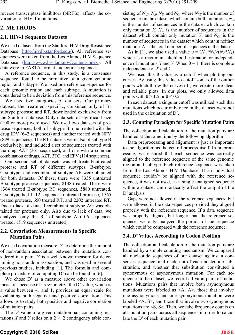

292 D. King et al. / J. Biomedical Science and Engineering 3 (2010) 291-299
reverse transcriptase inhibitors (NRTIs), affects the co-
variation of HIV-1 mutations.
2. METHODS
2.1. HIV-1 Sequence Datasets
We used datasets from the Stanford HIV Drug Resistance
Database (http://hivdb.stanford.edu/). All reference se-
quences were taken from the Los Alamos HIV Sequence
Database (http://www.hiv.lanl.gov /content/index). All
data were in FASTA-format nucleotide sequences.
A reference sequence, in this study, is a consensus
sequence, found to be normative of a given genomic
region and subtype. We used one reference sequence for
each genomic region and each subtype. A mutation is
considered to be a deviation from this reference sequence.
We used two categories of datasets. Our primary
dataset, the treatment-specific, consisted only of B-
subtype protease and RT, downloaded exclusively from
the Stanford database. Only data sets of significant size
(100 or more) were used. We used two datasets of pro-
tease sequences, both of subtype B, one treated with the
drug IDV (642 sequences) and another treated with NFV
(899 sequences). The RT datasets were also of subtype B
exclusively, and included a set of sequences treated with
the drug AZT (361 sequences), and one with a common
combination of drugs, AZT, 3TC, and EFV (114 sequences).
Our second set of datasets was of treated/untreated
protease and RT of different subtypes. B-subtype,
C-subtype, and recombinant subtype AE were obtained
for both datasets. Of these, there were 8335 untreated
B-subtype protease sequences, 8138 treated. There were
8364 treated B-subtype RT sequences, 5880 untreated.
C-subtype had 1112 sequences untreated protease, 1565
treated protease, 650 treated RT, and 2202 untreated RT.
Due to lack of data, Recombinant subtype AG was ob-
tained for protease only. Also due to lack of data, we
analyzed only the RT of subtype A (106 sequences
treated, 1519 sequences untreated).
2.2. Covariation Measurements in Specific
Mutation Pairs
We used covariation measure D’ to determine the amount
of non-random association between the mutations con-
sidered in a pair. D’ is a well known measure for deter-
mining non-random association, and was used in several
previous studies, including [1]. The formula and com-
plete procedure of computing D’ can be found in [6].
We chose D’ as a measure above other covariation
measures because of its symmetry: the D’ value, which is
a value between -1 and 1, provides an equal scale for
evaluating both negative and positive correlation. This
allows us to study both positive and negative correlation
of mutation pairs.
The D’ value of a given mutation pair containing mu-
tations X and Y relies on a 2 × 2 contingency table con-
sisting of NXY, NX, NY, and NO, where NXY is the number of
sequences in the dataset which contain both mutations, NX,
is the number of sequences in the dataset which contain
only mutation X, NY, is the number of sequences in the
dataset which contain only mutation Y, and NO, is the
number of sequences in the dataset which contain neither
mutation. N is the total number of sequences in the dataset.
As in [1], we also used a value θ = (Nxy*NO)/(NX*NY)
which is a maximum likelihood estimator for independ-
ence of mutations X and Y. When θ = 1, there is complete
independence of X and Y.
We used this θ value as a cutoff when plotting our
curves. By using this value to cutoff some of the outlier
points which throw the curves off, we create more clear
and reliable plots. In our plots, we only allowed data
points with θ > 1.5 or θ < 0.5.
In each dataset, a singular cutoff was utilized, such that
mutations which occur only once in the dataset were not
used in the calculation of D’.
2.3. Counting Paradigm for Specific Mutation Pairs
The collection and calculation of the mutation pairs are
handled at the same time by the following algorithm.
Data preprocessing and alignment is just as important
to the algorithm as the central process itself. In preproc-
essing, we ensured that each sequence was correctly
aligned to the reference sequence of the same genomic
region and subtype. Each reference sequence was taken
from the Los Alamos HIV Database. If an individual
sequence couldn’t be aligned with the reference se-
quence, it was not used, as a single unaligned sequence
within a dataset can drastically affect the output of the
D’ analysis.
Gaps were not allowed in the reference sequences, but
were allowed in the data sequences provided they aligned
properly with the reference sequence. If a data sequence
was properly aligned, but longer than the reference se-
quence, we only analyzed the portion of the sequence
which could be compared with the reference sequence.
2.4. D’ Values According to Codon Position
The collection and calculation of the mutation pairs are
handled by a simple counting mechanism. We compared
all nucleotide sequences of our dataset against a con-
sensus sequence, and made not of each nucleotide sub-
stitution, and whether that substitution constituted a
synonymous or asynonymous mutation. For each se-
quence in the dataset, we record all valid pairs of muta-
tions. Mutations pairs that involve both asynonymous
mutations were labeled as <A, A>, those that involve
one asynonymous and one synonymous mutation were
labeled <A, S>, and those that involve two synonymous
mutations are <S, S>. Then, we take frequency counts on
all mutation pairs across all sequences in order to calcu-
late the D’ of each mutation pair.

D. King et al. / J. Biomedical Science and Engineering 3 (2010) 291-299
293
JBiSE
For display, we use a sliding window curve. This en-
hances the readability and reliability of the curve. Sim-
ply graphing this data such that each physical position is
an average of all D’ values at that physical position give
an unsteady curve towards the greater physical distances.
As the physical distance increases, the number of data
points available for that physical distance decreases,
leading to greater oscillation as the plot goes on.
A sliding window has the same amount of data going
into each point on the graph, and is thus more reliable.
Our sliding window curves each use 3% of the data in
the set per window, with a 50% overlap.
2.5. D’ According to Genomic Position
We analyzed D’ according to amino acid position within
the genomic region as in [1]. This gives us information
on how specific codon positions interact with one an-
other within the gene, particularly in response to differ-
ent treatments.
We also performed a pair-wise analysis of these specific
mutation positions in order to reveal more on the differ-
ences between <A, A>, <A, S>, and <S, S> mutation pairs.
Using this data, we generated covariation histograms.
In these histograms, the value at each codon position is
the sum of the D’ value for all mutation pairs associated
with that position. Each mutation pair will contribute
total D’ value to the positions of its two mutations. In
this manner, positions which are either the site of great
amounts of mutation or high covariance will stand out,
with positions which are both high in mutation amount
and covariance being seen as peeks.
In order to further explore the relationships between
the amino acid positions, we cast our histograms into two
dimensional contour plots, which reveal clusters of co-
variation. To generate these plots, we form a square two
dimensional table with a length equal to the number of
amino acid positions in a given dataset. Each mutation
pair is then mapped to a position on this table, based on
the position of that pair’s mutations. For example, the
mutation pair L10I and Q20V would be mapped to posi-
tion x = 10, y = 20.
The value of each position in the table is the sum of
all D’ values of the pairs assigned to that position. This
provides a visual representation of the relationships be-
tween positions, with higher values representing posi-
tions which are highly correlated with one another, and
the lower values representing unrelated positions.
3. RESULTS
3.1. Effects of Specific Treatment on the
Covariation of B-Subtype Protease and RT
First, in order to discover the effects of specific treat-
ments on the covariation of HIV-1 mutation pairs, we
ran a D’ analysis on data sets of B-subtype protease and
RT with known treatment types. For reference, we also
included the generically treated and untreated datasets of
B-subtype protease and RT, in order to see how the dif-
ferent treatments effected the genomes and, and how the
compare to the effects of overall treatments.
Our findings revealed that covariation between muta-
tions is, as we expected, treatment dependent. In com-
paring IDV- and NFV-treated protease, these results
become clear. The plots in Figure 1, show the results of
the analysis according to physical distance, display
clearly different patterns in their covariation. The average
D’ values of <A, A> pair covariation are just at 0.3 for
both datasets, however we can clearly see peaks of high
covariance in different positions on the <A, A> curves. If
we compare these two treatment-specific plots against D’
values generated from the set of generically treated
HIV-1 sequences (those sequences that have received
treatment of any sort, plot not pictured), we can see that
the differences even more pronounced. The average D’ of
<A, A> mutation pairs in protease which has seen any
sort of treatment whatsoever is much higher—a value just
at 0.4, and yet a different set of peaks within the curve.
We see similar results in RT. The curves generated by RT
treated with the drug AZT are considerably different than
the generically treated RT, as can be seen in Figure 2.
The generic trends of covariation, however, were
largely the same despite what specific treatments were
used. <A, A> covariation tended to be higher than <A, S>
or <S, S> covariation in all datasets. In addition, we also
noticed that on average, <A, S> covariation tended to be
higher than <S, S>. This separation was even present in
the untreated dataset.
Figure 1. Different treatments lead to different patterns of
covariation. These two sliding window plots display the D’
analysis of two different treatment types. The top displays
results derived from IDV-based treatment, and the bottom plot
displays those derived from NFV. Clearly, the different treat-
ments induce quite different <A, A> covariation patterns in the
sliding window curves. The different treatments do not seem to
significantly affect the <A, S> or <S, S> curves.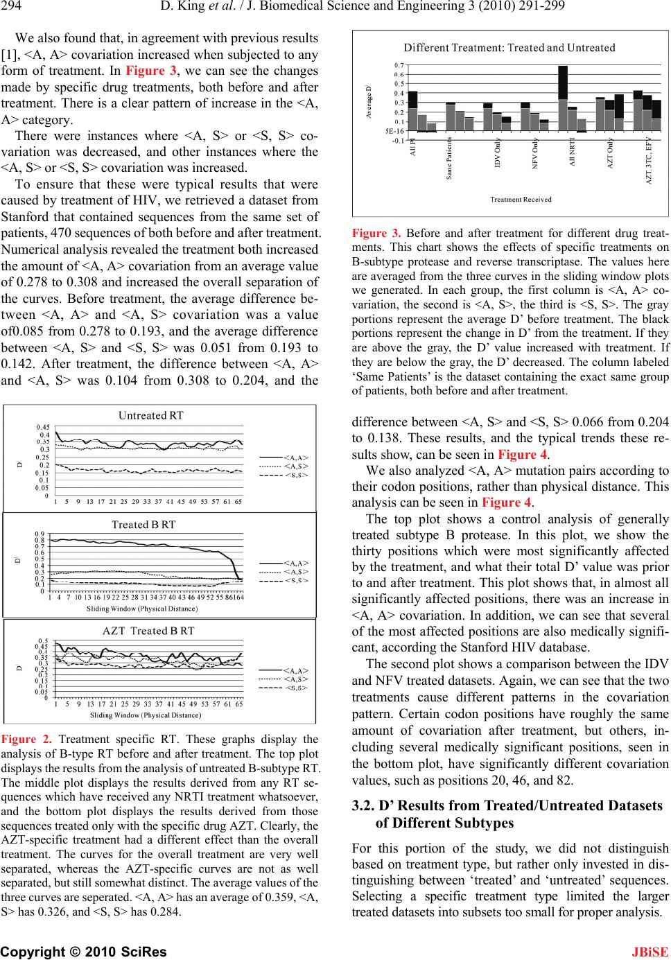

294 D. King et al. / J. Biomedical Science and Engineering 3 (2010) 291-299
To ensure that these were typical results that were
caused by treatment of HIV, we retrieved a dataset from
Stanford that contained sequences from the same set of
patients, 470 sequences of both before and after treatment.
Numerical analysis revealed the treatment both increased
the amount of <A, A> covariation from an average value
of 0.278 to 0.308 and increased the overall separation of
the curves. Before treatment, the average difference be-
tween <A, A> and <A, S> covariation was a value
of0.085 from 0.278 to 0.193, and the average difference
between <A, S> and <S, S> was 0.051 from 0.193 to
0.142. After treatment, the difference between <A, A>
and <A, S> was 0.104 from 0.308 to 0.204, and the
We also found that, in agreement with previous results
[1], <A, A> covariation increased when subjected to any
form of treatment. In Figure 3, we can see the changes
made by specific drug treatments, both before and after
treatment. There is a clear pattern of increase in the <A,
A> category.
There were instances where <A, S> or <S, S> co-
variation was decreased, and other instances where the
<A, S> or <S, S> covariation was increased.
Figure 2. Treatment specific RT. These graphs display the
analysis of B-type RT before and after treatment. The top plot
displays the results from the analysis of untreated B-subtype RT.
The middle plot displays the results derived from any RT se-
quences which have received any NRTI treatment whatsoever,
and the bottom plot displays the results derived from those
sequences treated only with the specific drug AZT. Clearly, the
AZT-specific treatment had a different effect than the overall
treatment. The curves for the overall treatment are very well
separated, whereas the AZT-specific curves are not as well
separated, but still somewhat distinct. The average values of the
three curves are seperated. <A, A> has an average of 0.359, <A,
S> has 0.326, and <S, S> has 0.284.
Figure 3. Before and after treatment for different drug treat-
ments. This chart shows the effects of specific treatments on
B-subtype protease and reverse transcriptase. The values here
are averaged from the three curves in the sliding window plots
we generated. In each group, the first column is <A, A> co-
variation, the second is <A, S>, the third is <S, S>. The gray
portions represent the average D’ before treatment. The black
portions represent the change in D’ from the treatment. If they
are above the gray, the D’ value increased with treatment. If
they are below the gray, the D’ decreased. The column labeled
‘Same Patients’ is the dataset containing the exact same group
of patients, both before and after treatment.
difference between <A, S> and <S, S> 0.066 from 0.204
to 0.138. These results, and the typical trends these re-
sults show, can be seen in Figure 4.
We also analyzed <A, A> mutation pairs according to
their codon positions, rather than physical distance. This
analysis can be seen in Figure 4.
The top plot shows a control analysis of generally
treated subtype B protease. In this plot, we show the
thirty positions which were most significantly affected
by the treatment, and what their total D’ value was prior
to and after treatment. This plot shows that, in almost all
significantly affected positions, there was an increase in
<A, A> covariation. In addition, we can see that several
of the most affected positions are also medically signifi-
cant, according the Stanford HIV database.
The second plot shows a comparison between the IDV
and NFV treated datasets. Again, we can see that the two
treatments cause different patterns in the covariation
pattern. Certain codon positions have roughly the same
amount of covariation after treatment, but others, in-
cluding several medically significant positions, seen in
the bottom plot, have significantly different covariation
values, such as positions 20, 46, and 82.
3.2. D’ Results from Treated/Untreated Datasets
of Different Subtypes
For this portion of the study, we did not distinguish
based on treatment type, but rather only invested in dis-
tinguishing between ‘treated’ and ‘untreated’ sequences.
Selecting a specific treatment type limited the larger
treated datasets into subsets too small for proper analysis.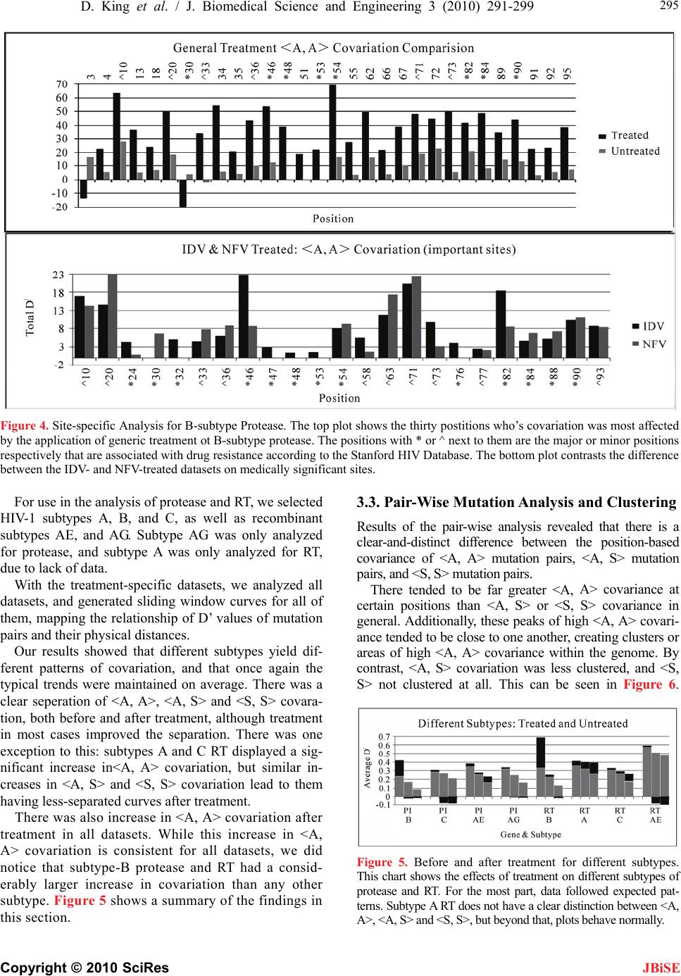

D. King et al. / J. Biomedical Science and Engineering 3 (2010) 291-299
295
Figure 4. Site-specific Analysis for B-subtype Protease. The top plot shows the thirty postitions who’s covariation was most affected
by the application of generic treatment ot B-subtype protease. The positions with * or ^ next to them are the major or minor positions
respectively that are associated with drug resistance according to the Stanford HIV Database. The bottom plot contrasts the difference
between the IDV- and NFV-treated datasets on medically significant sites.
3.3. Pair-Wise Mutation Analysis and Clustering
For use in the analysis of protease and RT, we selected
HIV-1 subtypes A, B, and C, as well as recombinant
subtypes AE, and AG. Subtype AG was only analyzed
for protease, and subtype A was only analyzed for RT,
due to lack of data.
Results of the pair-wise analysis revealed that there is a
clear-and-distinct difference between the position-based
covariance of <A, A> mutation pairs, <A, S> mutation
pairs, and <S, S> mutation pairs.
With the treatment-specific datasets, we analyzed all
datasets, and generated sliding window curves for all of
them, mapping the relationship of D’ values of mutation
pairs and their physical distances.
There tended to be far greater <A, A> covariance at
certain positions than <A, S> or <S, S> covariance in
general. Additionally, these peaks of high <A, A> covari-
ance tended to be close to one another, creating clusters or
areas of high <A, A> covariance within the genome. By
contrast, <A, S> covariation was less clustered, and <S,
S> not clustered at all. This can be seen in Figure 6.
Our results showed that different subtypes yield dif-
ferent patterns of covariation, and that once again the
typical trends were maintained on average. There was a
clear seperation of <A, A>, <A, S> and <S, S> covara-
tion, both before and after treatment, although treatment
in most cases improved the separation. There was one
exception to this: subtypes A and C RT displayed a sig-
nificant increase in<A, A> covariation, but similar in-
creases in <A, S> and <S, S> covariation lead to them
having less-separated curves after treatment.
There was also increase in <A, A> covariation after
treatment in all datasets. While this increase in <A,
A> covariation is consistent for all datasets, we did
notice that subtype-B protease and RT had a consid-
erably larger increase in covariation than any other
subtype. Figure 5 shows a summary of the findings in
this section.
Figure 5. Before and after treatment for different subtypes.
This chart shows the effects of treatment on different subtypes of
protease and RT. For the most part, data followed expected pat-
terns. Subtype A RT does not have a clear distinction between <A,
A>, <A, S> and <S, S>, but beyond that, plots behave normally.
JBiSE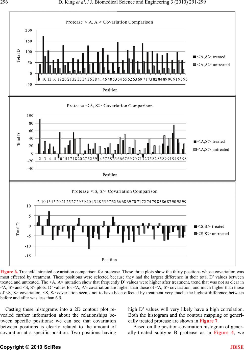

296 D. King et al. / J. Biomedical Science and Engineering 3 (2010) 291-299
Figure 6. Treated/Untreated covariation comparison for protease. These three plots show the thirty positions whose covariation was
most effected by treatment. These positions were selected because they had the largest difference in their total D’ values between
treated and untreated. The <A, A> mutation show that frequently D’ values were higher after treatment, trend that was not as clear in
<A, S> and <S, S> plots. D’ values for <A, A> covariation are higher than those of <A, S> covariation, and much higher than those
of <S, S> covariation. <S, S> covariation seems not to have been effected by treatment very much: the highest difference between
before and after was less than 6.5.
Casting these histograms into a 2D contour plot re-
vealed further information about the relationships be-
tween specific positions: we can see that covariation
between positions is clearly related to the amount of
covaration at a specific position. Two positions having
high D’ values will very likely have a high correlation.
Both the histogram and the contour mapping of generi-
cally treated protease are shown in Figure 7.
Based on the position-covariation histogram of gener-
ally-treated subtype B protease as in Figure 4, we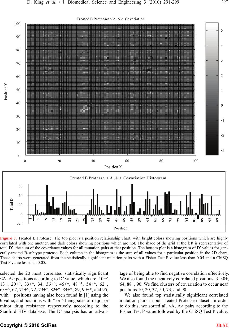

D. King et al. / J. Biomedical Science and Engineering 3 (2010) 291-299
297
JBiSE
Figure 7. Treated B Protease. The top plot is a position relationship chart, with bright colors showing positions which are highly
correlated with one another, and dark colors showing positions which are not. The shade of the grid at the left is representative of
total D’, the sum of the covariance values for all mutation pairs at that position. The bottom plot is a histogram of D’ values for gen-
erally-treated B-subtype protease. Each column in the histogram is the sum of all values for a particular position in the 2D chart.
These charts were generated from the statistically significant mutation pairs with a Fisher Test P value less than 0.05 and a ChiSQ
Test P value less than 0.05.
selected the 20 most correlated statistically significant
<A, A> positions according to D’ value, which are: 10+^,
13+, 20+^, 33+^, 34, 36+^, 46+*, 48+*, 54+*, 62+,
63+^, 67, 71+^, 72, 73+^, 82+*, 84+*, 89, 90+*, and 95,
with + positions having also been found in [1] using the
θ value, and positions with * or ^ being sites of major or
minor drug resistance respectively according to the
Stanford HIV database. The D’ analysis has an advan-
tage of being able to find negative correlation effectively.
We also found the negatively correlated positions: 3, 30+,
64, 88+, 96. We find clusters of covariation to occur near
positions 10, 20, 37, 50, 73, and 90.
We also found top statistically significant correlated
mutation pairs in our Treated Protease dataset. In order
to do this, we sorted all <A, A> pairs according to the
Fisher Test P value followed by the ChiSQ Test P value,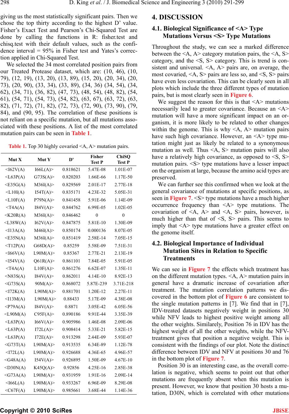

298 D. King et al. / J. Biomedical Science and Engineering 3 (2010) 291-299
giving us the most statistically significant pairs. Then we
chose the top thirty according to the highest D’ value.
Fisher’s Exact Test and Pearson’s Chi-Squared Test are
done by calling the functions in R: fisher.test and
chisq.test with their default values, such as the confi-
dence interval = 95% in Fisher test and Yates’s correc-
tion applied in Chi-Squared Test.
We selected the 34 most correlated position pairs from
our Treated Protease dataset, which are: (10, 46), (10,
79), (12, 19), (13, 20), (13, 89), (15, 20), (20, 34), (20,
73), (20, 90), (33, 34), (33, 89), (34, 36) (34, 54), (34,
62), (34, 71), (36, 82), (47, 73), (48, 54), (48, 82), (54,
61), (54, 71), (54, 73), (54, 82), (63, 67), (63, 72), (63,
82), (71, 72), (71, 82), (72, 73), (72, 90), (73, 90), (79,
84), and (90, 95). The correlation of these positions is
not reliant on a specific mutation, but all mutations asso-
ciated with these positions. A list of the most correlated
mutation pairs can be seen in Table 1.
Table 1. Top 30 highly covaried <A, A> mutation pairs.
Mut X Mut Y D' Fisher
Test P
ChiSQ
Test P
<I62V(A) I66L(A)> 0.818621 5.47E-08 1.01E-07
<L63P(A) G73S(A)> 0.820203 1.66E-66 1.17E-50
<E35G(A) M36I(A)> 0.829569 2.01E-17 2.77E-18
<L10I(A) I54T(A)> 0.835171 4.23E-32 5.05E-31
<L10F(A) P79N(A)> 0.841458 5.91E-06 1.14E-09
<T4A(A) I84V(A)> 0.844762 6.99E-05 1.02E-05
<K20R(A) M36I(A)> 0.846462 0 0
<L38W(A) I62V(A)> 0.847875 5.81E-10 1.30E-09
<I13A(A) M46I(A)> 0.850174 0.000136 8.07E-05
<E35N(A) M36I(A)> 0.851419 2.58E-14 7.05E-15
<T12P(A) G68D(A)> 0.85259 5.58E-09 7.51E-31
<I66V(A) L90M(A)> 0.85367 2.77E-21 2.13E-19
<I54V(A) Q61R(A)> 0.861101 7.84E-05 5.91E-05
<T4A(A) L10F(A)> 0.861276 6.62E-07 1.35E-11
<N83S(A) I84V(A)> 0.862011 4.14E-10 8.92E-13
<G73S(A) 90M(A)> 0.868072 5.87E-239 3.71E-218
<I72K(A) L90M(A)> 0.881701 1.20E-12 2.27E-11
<I13M(A) L90M(A)> 0.88433 5.17E-09 4.38E-08
<P79A(A) I84V(A)> 0.8871 3.05E-42 6.05E-56
<L90M(A) C95F(A)> 0.890186 9.91E-44 3.35E-39
<L63P(A) I66V(A)> 0.905986 1.46E-08 2.09E-06
<L63P(A) I72L(A)> 0.908414 5.33E-21 5.82E-15
<L63P(A) I72E(A)> 0.913298 2.44E-09 5.93E-07
<G73T(A) L90M(A)> 0.913535 6.34E-89 1.12E-78
<I72L(A) L90M(A)> 0.926688 4.36E-65 4.96E-57
<G48A(A) I54V(A)> 0.926895 1.50E-09 4.67E-10
<D30N(A) K45Q(A)> 0.92856 4.25E-16 2.85E-38
<G73A(A) L90M(A)> 0.931959 1.91E-16 2.09E-14
<I66L(A) L90M(A)> 0.933267 6.96E-09 8.29E-08
<C67F(A) L90M(A)> 0.985661 3.68E-44 1.14E-36
4. DISCUSSION
4.1. Biological Significance of <A> Type
Mutations Versus <S> Type Mutations
Throughout the study, we can see a marked difference
between the <A, A> category mutation pairs, the <A, S>
category, and the <S, S> category. This is trend is con-
sistent and universal. <A, A> pairs are, on average, the
most covaried, <A, S> pairs are less so, and <S, S> pairs
have even less covariation. This can be clearly seen in all
plots which include the three different types of mutation
pairs, but is most clearly seen in Figure 6.
We suggest the reason for this is that <A> mutations
necessarily lead to greater covariance. Because an <A>
mutation will have a more significant impact on an or-
ganism, it is more likely to be related to other changes
within the genome. This is why <A, A> mutation pairs
have such high covariance. However, an <A> type mu-
tation might just as likely be related to a synonymous
mutation as well. Thus <A, S> mutation pairs will also
have a relatively high covariance, as opposed to <S, S>
mutation pairs. <S> type mutations have a lesser impact
on the organism at large, because the amino acid types are
preserved.
We can further see this confirmed when we look at the
general covariance of mutations at specific positions, as
seen in Figure 7. <S> type mutations have a much higher
occurrence frequency than <A> type mutations. The
covariation of <A, A> and <A, S> pairs, however, is
much higher than that of <S, S> pairs. This seems to
imply that <A> type mutations have a greater effect on
the genome itself.
4.2. Biological Importance of Individual
Mutation Sites in Relation to Specific
Treatments
We can see in Figure 7 the effects which treatment has
on the different mutation types. <A, A> mutation pairs in
general have a dramatic increase of covariation after
treatment. The mutation correlation patterns we dis-
covered in the bottom plot of Figure 6 are consistent to
the single mutation patterns in [7]. We find that in [7],
IDV-treated datasets negatively weight in positions 30
while NFV leads to highest positive weight among all
the other weights. Similarely, Position 76 in IDV has the
highest weight of all the other weights, while the NFV-
treatment gives that position a negative weight. This is
consistent with the findings of our plot. Note the distinct
difference between IDV and NFV at positions 30 and 76
in the bottom plot of Figure 7.
Position 30 is an interesting case, as the overall corre-
lation is negative, which seems to point out that other
mutations are frequently absent when this mutation is
present. However, we know that position 30 hosts a mu-
tation, D30N, which is correlated with other mutations

D. King et al. / J. Biomedical Science and Engineering 3 (2010) 291-299
299
when the specific PI treatment is neflinavir. This seems
to hint that other treatment types have a steep inverse
correlation at this mutation site. At the very least, we see
that the treatment IDV gives a negative correlative
weight at position 30 [7].
JBiSE
4.3. Differences in Covariation in Different
Treatments and Subtypes
While the general trends we found were largely consis-
tent throughout our comparison between the different
treatments and subtypes, we found the differences in the
covariation patterns between the subtypes and treatments
interesting.
In Figure 4, we see that the increase in covariation
between the untreated sequences and the the sequences
which received any treatment whatsoever is far larger
than the increase in covariation present in those se-
quences only treated with individual drugs. For example,
the two drugs, NFV and IDV, have the most data within
the Stanford database. In spite of this, neither the co-
variation increase from NFV or IDV alone is enough to
cause the dramatic increase we see from generic treat-
ment of B-subtype protease. The same is true of AZT-
treated RT compared with generically treated RT. The
generically treated datasets accounts for sequences
treated with single drugs, such as NFV or IDV or AZT,
as well as those treated with combinations of drugs. Our
results, then, suggest that combinations of treatments
lead to greater covariance than single treatments. This is
further supported by the results of the RT treated with
the combination of drugs, AZT, 3TC, and EFV, which
have a greater increase in covariation than any single-
treatment, but still not as much as the generically-treated
sequences.
5. ACKNOWLEDGEMENTS
We would like to thank Houghton College for providing the funding for
this research through the Summer Research Institute at Houghton, as
well as Qi Wang for responding to our e-mails regarding his paper [1]
both promptly and helpfully.
REFERENCES
[1] Wang, Q. and Lee, C. (2007) Distinguishing functional
amino acid covariation from background linkage disequi-
librium in HIV protease and reverse transcriptase. PLoS
ONE, 2(8), 814.
[2] Liu, Y., Eyal, E. and Bahar, I. (2008) Analysis of corre-
lated mutations in HIV-1 protease using spectral cluster-
ing. Bioinformatics, 24, 1243-1250.
[3] Gilbert, P.B., Novitsky, V. and Essex, M. (2005) Covari-
ability of selected amino acid positions for HIV type 1
subtypes C and B. AIDS Research and Human Retrovi-
ruses, 21(12), 1016-1030
[4] Hoffman, N.G., Schiffer, C.A. and Swanstrom, R. (2003)
Covariation of amino acid positions in HIV-1 protease.
Virology, 314, 536-548.
[5] Rhee, S.Y., Liu, T.F., Holmes, S.P. and Shafer, R.W.
(2007) HIV-1 subtype B protease and reverse transcrip-
tase amino acid covariation. PLoS Computational Biol-
ogy, 3(5), 87.
[6] Hedrick, P. (1987) Gametic disequilibrium measure:
proceed with caution. Genetics, 117, 331-341.
[7] Rhee, S.Y., Taylor, J., Wadhera, G., Ben-Hur, A., Brutlag,
D. and Shafer, R.W. (2006) Genotypic predictors of hu-
man immunodeficiency virus type 1 drug resistance.
Proceedings of the National Academy of Sciences USA.
103, 17355-17360.
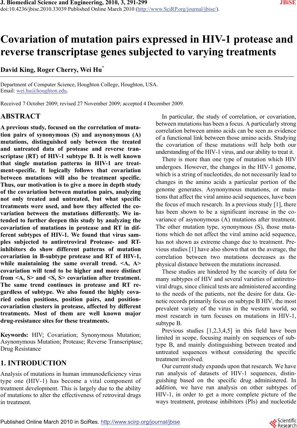