J. Software Engineer & Applications, 2010, 3: 191-197
doi:10.4236/jsea.2010.33024 Published Online March 2010 (http://www.SciRP.org/journal/jsea)
191
Linear Control Problems of the Fuzzy Maps
Andrej V. Plotnikov, Tatyana A. Komleva, Irina V. Molchanyuk
Department of Applied Mathematics, Odessa State Academy of Civil Engineering and Architecture, Odessa, Ukraine.
Received October 28th, 2009; revised November 16th, 2009; accepted November 20th, 2009.
ABSTRACT
In the present paper, we show the some properties of the fuzzy R-solution of the control linear fuzzy differential inclu-
sions and research the optimal time problems for it.
Keywords: Fuzzy Differential Inclusions, Control Problems
1. Introduction
The first study of differential equations with multivalued
right-hand sides was performed by A. Marchaud [1] and
S. C. Zaremba [2]. In early sixties, T. Wazewski [3,4], A.
F. Filippov [5] obtained fundamental results on existence
and properties of the differential equations with multi-
valued right-hand sides (differential inclusions). One of
the most important results of these articles was an estab-
lishment of the relation between differential inclusions
and optimal control problems, that promoted to develop
the differential inclusion theory [6–9].
Considering of the differential inclusions required to
study properties of multivalued functions, i.e. an elab-
oration the whole tool of mathematical analysis for mul-
tivalued functions [6,10,11].
In works [12,13] annotate of an R-solution for differ-
ential inclusion is introduced as an absolutely continuous
multivalued function. Various problems for the R-solu-
tion theory were regarded in [14–18]. The basic idea for
a development of an equation for R-solutions (integral
funnels) is contained in [19].
In the last years there has been forming new approach
to control problems of dynamic systems, which founda-
tion on analysis of trajectory bundle but not separate tra-
jectories. The section of this bundle in any instant is
some set and it is necessary to describe the evolution of
this set. Obtaining and research dynamic equations of
sets there is important problem in this case. The metric
space of sets with the Hausdorff metric is natural space
for description dynamic of sets. In theory of multivalued
maps definitions on derivative as for single-valued maps
is impossible because space of sets is nonlinear. This
bound possibility description dynamic sets by differential
equations. Therefore, the control differential equations with
set of initial conditions [20–22] and the control differen-
tial inclusions [8,23–34] use for it.
In recent years, the fuzzy set theory introduced by
Zadeh [35] has emerged as an interesting and fascinating
branch of pure and applied sciences. The applications of
fuzzy set theory can be found in many branches of re-
gional, physical, mathematical, differential equations,
and engineering sciences. Recently there have been new
advances in the theory of fuzzy differential equations
[36–47] and inclusions [43,48–52] as well as in the the-
ory of control fuzzy differential equations [53–55] and
inclusions [56,57].
In this article we consider the some properties of the
fuzzy R-solution of the control linear fuzzy differential
inclusions and research the optimal time problems for it.
2. The Fundamental Definitions and
Designations
Let






nn RconvRcomp be a set of all nonempty (con-
vex) compact subsets from the space Rn,



 ABSBASBAh rr
r

)(,)(min,0
be Hausdorff distance between sets A and B, Sr(A) is
r
-neighborhood of set A.
Let En be the set of all u: Rn→[0,1] such that u satisfies
the following conditions:
1) u is normal, that is, there exists an such
that u(x0)=1;
n
Rx 
0
2) u is fuzzy convex, that is,

 )(),(min)1( yuxuyxu  




;
3) For any and
n
Ryx,10 

;
4) u is upper semicontinuous;

Linear Control Problems of the Fuzzy Maps 192
5) is compact.
  0)(:
0 xuRxclu n
If , then u is called a fuzzy number, and En is
said to be a fuzzy number space. For
n
Eu 
10 

, denote





 )(: xuRxu n.
Then from 1)-4), it follows that the α-level set
 for all  
n
Rconvu 

10



.
Theorem 1. (Negoita and Ralescu [58]). If ,
then
n
Eu 
1) for all
 
n
Rconvu 

 ]1,0[

;
2) for  

uu 10 




;
3) If

]1,0[
k

is a decreasing sequence converg-
ing to 0

then
 

1

k
k
uu

Conversely, if is a family of convex
compact subsets of satisfying 1)-3), then
 10:  

A
n
R





Au 
for 10 

and

0
10
0AAu 




.
If is a function, then using Zadeh’s
extension principle we can extend g
nnnRRRg :
~
to
by the equation
nnn EEE 
 )(),(minsup))(,(
~
),(
yvxuzvug
yxgz 
.
It is well known that




vugvug ,),(
~

for all and continuous function 10,,  
n
Evu
g
.
Further, we have


vuvu  , ,  

ukku 
where . Rk 
Define by the relation
),0[:  nn EED
 



vuhvuD ,sup),(
10 
,
where h is the Hausdorff metric defined in comp(Rn).
Then D is a metric in En.
Further we know that [59]
1) (En,D) is a complete metric space;
2) for all ;
 vuDwvwuD ,,  
n
Ewvu,,
3)
  vuDvuD ,,   
for all and
n
Evu ,
R

.
It can be proved that

 ),(),(, zvDwuDzwvuD




for .
n
Ezwvu ,,,
Definition 1. A mapping is strongly
measurable if for all
n
ETF ],0[:
]1,0[


the set-valued map


n
RconvTF ],0[:

defined by



)(tF

)(tF  is
Lebesgue measurable.
Definition 2. A mapping is said to be
integrably bounded if there is an integrable function
such that
n
ETF ],0[:
)(th )()( thtx for every . )(
0tF)(tx
Definition 3. The integral of a fuzzy mapping


n
ETF ,0:

T
dttF
0
)(

n
RTf ],0[:
is defined levelwise by
The set of allsuch that
is a measurable selection for for all







T
dttF
0
)(

F

T
dttf
0
)(

 1,0


.
Definition 4. A strongly measurable and integrably
bounded mapping


n
ETF ,0: is said to be inte-
grable over

 T,0 if .

Tn
EdttF
0
)(
Note that if


n
ETF ,0: is strongly measurable
and integrably bounded, then F is integrable. Further if


n
ETF ,0: is continuous, then it is integrable.
Theorem 2. [36]. Let be integrable
and

n
ETGF,0:,

 Tc ,0

,R


. Then
1)




TT
c
c
dttFdttFdttF
00
;)()()(
2) ;




TTT
dttGdttFdttGtF
000
)()()()(
3) ;


TT
dttFdttF
00
)()( 
4)


GFD , is integrable;
5)
 dttGtFDdttGdttFD
TTT 







000
)(),()(,)(
Consider the following control linear fuzzy differential
inclusions
,)(),,()( 00xtxwtGxtAx


 (1)
and the following nonlinear fuzzy differential inclusions
,)(),,,(00 xtxwxtFx 

 (2)
where means x
dt
dx ; 

Rt is the time; is
the state; is the control; is
n
Rx 
m
Rw )(tA


nn

-di-
mensional matrix-valued function; ,
are the set-valued functions.
n

mER RG :
n
ERF  :mn RR
Let

Linear Control Problems of the Fuzzy Maps193
)(: m RconvRW 
 (3)
be the measurable multivalued map.
Definition 5. Set of all single-valued branches
of the multivalued map is the set of the possible
controls.
LW
W


Obviously, the control fuzzy differential Inclusion (2)
turns into the ordinary fuzzy differential inclusion
 ,)(,, 00 xtxxtx 
 (4)
if the control

LWw 
~
is fixed and




xt,
 )(
~
,, twxtF .
The fuzzy differential Inclusions (3) has the fuzzy
R-solution, if right-hand side of the fuzzy differential
Inclusion (3) satisfies some conditions [52].
Let denotes the fuzzy R-solution of the differ-
ential Inclusion (3), then denotes the fuzzy
R-solution of the control differential Inclusion (2) for the
fixed .
)(tX
 w
),(wtX
LW
Definition 6. The set
 LWwwTXTY :,)( 
be called the attainable set of the fuzzy System (2).
3. The Some Properties of the R-Solution
In this section, we consider the some properties of the
R-solution of the control fuzzy differential Inclusion (1).
Let the following condition is true.
Condition A:
A1. is measurable on  A

 Tt ,
0;
A2. The norm
 tA of the matrix is inte-
grable on ;
 tA
 Tt ,
0
A3. The multivalued map



m
RconvTtW,: 0 is
measurable on ;

Tt,
0
A4. The fuzzy map satisfies the
conditions
nm ERRG 

:
1) measurable in t;
2) continuous in w;
A5. There exist


 TtLv ,
02
 and 

 TtLl ,
02


such that
  tlwtGtvtW  ,,
almost everywhere on ;  Tt ,
0
A6. The set is compact
and convex for almost every , i.e.
.

LWwtwtGtQ :)(,
 t,
0
)
n



T
()( EconvtQ 
Theorem 3. Let the condition A is true.
Then for every there exists the fuzzy
R-solution such that
 LWw 

wX ,
1) the fuzzy map

 wX ,

has form
 
0
1
0
,ΦΦΦ() (, ())
t
t
X
twt xtsGswsds


,
where

 Ttt ,
0

;

 t

is Cauchy matrix of the differ-
ential equation xtA )(x

;
2) for every ;
n
EwtX ),(  Ttt,
0

3) the fuzzy map


wX ,

is the absolutely continuous
fuzzy map on

 . Tt ,
0
Proof. The proof is easy consequence of the
[31,34,52,54] and Theorem 1.
Theorem 4. Let the condition A is true.
Then the attainable set is compact and convex.  TY
Proof. The proof is easy consequence of the
[31,34,52,54] and Theorem 1.
We obtained the basic properties of the fuzzy
R-solution of System (1). Now, we consider the some
control fuzzy problems.
4. The Optimal Time Problems
Consider the control linear fuzzy differential Inclusion
(1), when
)()(),(tFwtBwtG 

, (4)
where
B1.



B is measurable on  ; Tt ,
0
B2. The norm

 tB of the matrix is inte-
grable on

tB

 Tt,
0;
B3. The fuzzy map F: [t0,T]→En is measurable on
[t0,T];
B4. There exists

  TtLf ,
02



such that

 tftF
almost everywhere on [t0,T].
Consider the following optimal control problem: it is
necessary to find the minimal time
T
and the control

 LWw 
* such that the fuzzy R-solution of Systems
(1),(4) satisfies one of the conditions:



k
SwTX 
*
,, (5)


k
SwTX
*
,, (6)


k
SwTX 
*
,, (7)
where is the terminal set.
n
kES 
Clearly, these time optimal problems are different from
the ordinary time optimal problem by that here control
object has the volume.
Definition 6. We shall say that the pair






**,, wXw 
 satisfies the maximum principle on , if there exists
the vector-function
 Tt ,
0




, which is the solution of the

Linear Control Problems of the Fuzzy Maps 194
system
 )0(,)( 1 STtAT 

and the following conditions are true
1) the maximum condition


 )(,)(max)(),()( )(
*twtBCttwtBC tWw



almost everywhere on ;
 Tt ,
0
2) the transversal condition:
a) in the case (5):



11
*
(,), (),()
k
CXTw ψTCSψT


 ;
b) in the case (6): for all  1,0






*
(,), (),
αα
k
CXTw ψTCSψT


and there exists

1,0

such that


 

*
(,) ,,
ββ
k
CXTwψTCSψT

 ;
c) in the case (6): for all  1,0





*
(,), (), ()
αα
k
CXTwψTCS ψT

 

and there exists

1,0

such that



*
(,), (), ()
ββ
k
CXTw ψTCS ψT

 
 .
Clearly, that there cases of the transversal condition of
the maximum principle correspond to the three cases of
the time optimal problems.
Theorem 5. (necessary optimal condition). Let the
condition A are true and the pair 



*
,wT is optimality.
Then the pair 




**,,wXw satisfies the maximum
principle on.

Tt ,
0
Proof. Let is the optimal control and


*
w


*
,wX
is the optimal R-solution of the Systems (1),(4), i.e.
1)


 ;, *TYwTX 
2)


., *
k
SwTX 
From 1) and 2) we have




1
1
max ,,
k
XYT
CXψCS ψ



for all )0(
1
S

.
Consequently
 
 

11
1
0
max min,,0.
k
ψS
XYT
pCXψCSψ




From


11
*
,k XTw S




 we have
 



11
*
,,,,
k
qTψCXTw ψCSψ



for all


0
1
S


.
From Theorem 1 we have that the function



,Tq is
continuous on )0(
1
SR

.
If


0, 

Tq for all

0
1
S

then we have





0,qT Tψγ
10
min
ψSq 0

. Hence there exists T


such that

 0
0
 q. Consequently we have





11
*
,, ,
k
CXτwψCS ψ


 0
for all

 0
1
S


, i.e. .


11
*
,k XτwS




It contradicts that is optimal time. T
If , 0p


 




11
1
0
()
1
max min,,
,,
k
ψS
XYT
k
CXψCS ψ
CXψCS ψ




and




XwTX
~
,1
*, than we have a contradiction.
Hence there exist


0
~
1
S


such that





1
1
*
,, max,
XYT
CXTw ψCXψ
 





,





1
*
,, ,
k
CXTw ψCS ψ




1.
Consequently
 
1*
0
ΦΦ ,
T
TsBsw sdsψ






 
1
0
max ΦΦ ,
T
wLW T sBswsdsψ






Then we have








1*
ΦΦ ,TsBswsψ



 


1
max ΦΦ ,
wLW TsBswsψ



for almost everywhere

 Tts,
0

. If
  


 

1
1
ΦΦ
ΦΦ
T
T
Ttψ
ψt
Ttψ



,
than the theorem is proved.
Example. Consider the following control linear fuzzy
differential inclusions
,0)0(,
01
10 









xFwxx

0
where


T
xxx 21 , is the state;
is the control;
 
12 1
,0
T
www WS

2
E
F

is the fuzzy set, where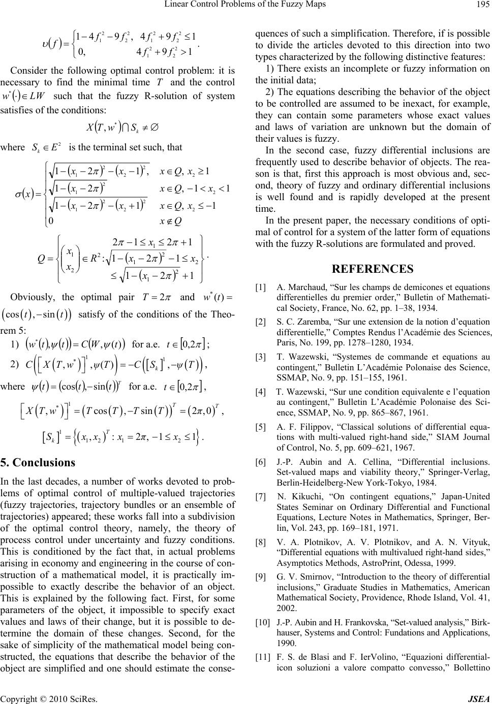

Linear Control Problems of the Fuzzy Maps195






194,0
194,941
2
2
2
1
2
2
2
1
2
2
2
1
ff
ffff
f  .
Consider the following optimal control problem: it is
necessary to find the minimal time
T
and the control
such that the fuzzy R-solution of system
satisfies of the conditions:
 LWw
*



k
SwTX 
*
,
where is the terminal set such, that
2
ESk
















Qx
xQxxx
xQxx
xQxxx
x
0
1,121
11,21
1,,121
2
2
2
2
1
2
2
1
2
2
2
2
1





























121
121
1212
:
2
1
2
2
1
1
2
2
1



x
xx
x
R
x
x
Q.
Obviously, the optimal pair

2T and *()wt

satisfy of the conditions of the Theo-
rem 5:
 

cos,sint

t

1) for a.e.
    )(,,
*tWCttw
 


2,0t;
2) ,





11
*
,,(),
k
CXTw ψTCSψT



where for a.e.  
T
ttt sin,cos  

2,0t,

   
1
*
,cos,sin2,
TT
XTwTTTTπ


 0,





1
12 12
,: 2,11
T
k
Sxxxπx.
5. Conclusions
In the last decades, a number of works devoted to prob-
lems of optimal control of multiple-valued trajectories
(fuzzy trajectories, trajectory bundles or an ensemble of
trajectories) appeared; these works fall into a subdivision
of the optimal control theory, namely, the theory of
process control under uncertainty and fuzzy conditions.
This is conditioned by the fact that, in actual problems
arising in economy and engineering in the course of con-
struction of a mathematical model, it is practically im-
possible to exactly describe the behavior of an object.
This is explained by the following fact. First, for some
parameters of the object, it impossible to specify exact
values and laws of their change, but it is possible to de-
termine the domain of these changes. Second, for the
sake of simplicity of the mathematical model being con-
structed, the equations that describe the behavior of the
object are simplified and one should estimate the conse-
quences of such a simplification. Therefore, if is possible
to divide the articles devoted to this direction into two
types characterized by the following distinctive features:
1) There exists an incomplete or fuzzy information on
the initial data;
2) The equations describing the behavior of the object
to be controlled are assumed to be inexact, for example,
they can contain some parameters whose exact values
and laws of variation are unknown but the domain of
their values is fuzzy.
In the second case, fuzzy differential inclusions are
frequently used to describe behavior of objects. The rea-
son is that, first this approach is most obvious and, sec-
ond, theory of fuzzy and ordinary differential inclusions
is well found and is rapidly developed at the present
time.
In the present paper, the necessary conditions of opti-
mal of control for a system of the latter form of equations
with the fuzzy R-solutions are formulated and proved.
REFERENCES
[1] A. Marchaud, “Sur les champs de demicones et equations
differentielles du premier order,” Bulletin of Mathemati-
cal Society, France, No. 62, pp. 1–38, 1934.
[2] S. C. Zaremba, “Sur une extension de la notion d’equation
differentielle,” Comptes Rendus l’Académie des Sciences,
Paris, No. 199, pp. 1278–1280, 1934.
[3] T. Wazewski, “Systemes de commande et equations au
contingent,” Bulletin L’Académie Polonaise des Science,
SSMAP, No. 9, pp. 151–155, 1961.
[4] T. Wazewski, “Sur une condition equivalente e l’equation
au contingent,” Bulletin L’Académie Polonaise des Sci-
ence, SSMAP, No. 9, pp. 865–867, 1961.
[5] A. F. Filippov, “Classical solutions of differential equa-
tions with multi-valued right-hand side,” SIAM Journal
of Control, No. 5, pp. 609–621, 1967.
[6] J.-P. Aubin and A. Cellina, “Differential inclusions.
Set-valued maps and viability theory,” Springer-Verlag,
Berlin-Heidelberg-New York-Tokyo, 1984.
[7] N. Kikuchi, “On contingent equations,” Japan-United
States Seminar on Ordinary Differential and Functional
Equations, Lecture Notes in Mathematics, Springer, Ber-
lin, Vol. 243, pp. 169–181, 1971.
[8] V. A. Plotnikov, A. V. Plotnikov, and A. N. Vityuk,
“Differential equations with multivalued right-hand sides,”
Asymptotics Methods, AstroPrint, Odessa, 1999.
[9] G. V. Smirnov, “Introduction to the theory of differential
inclusions,” Graduate Studies in Mathematics, American
Mathematical Society, Providence, Rhode Island, Vol. 41,
2002.
[10] J.-P. Aubin and H. Frankovska, “Set-valued analysis,” Birk-
hauser, Systems and Control: Fundations and Applications,
1990.
[11] F. S. de Blasi and F. IerVolino, “Equazioni differential-
icon soluzioni a valore compatto convesso,” Bollettino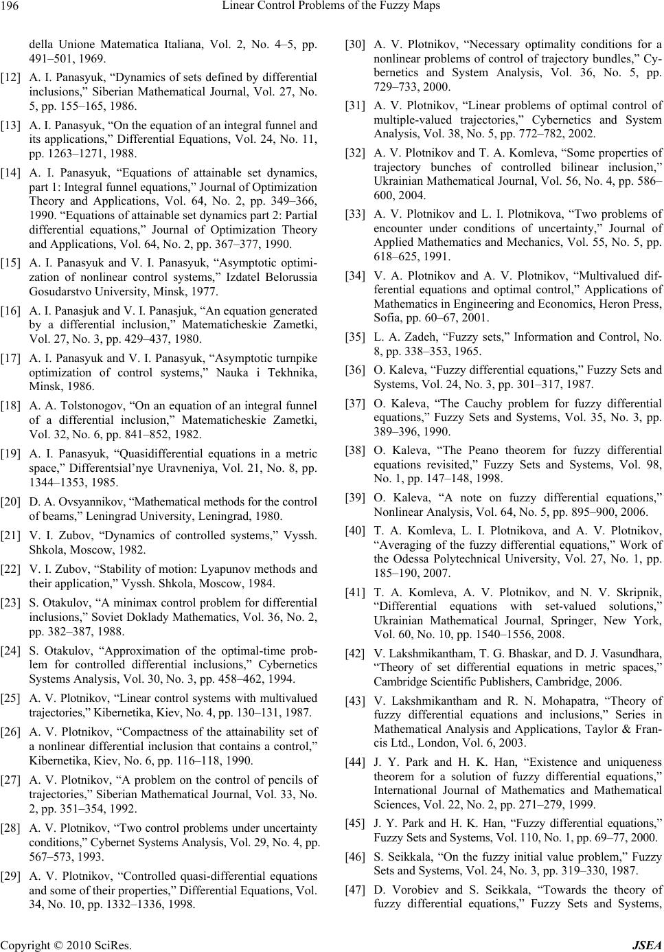

Linear Control Problems of the Fuzzy Maps 196
della Unione Matematica Italiana, Vol. 2, No. 4–5, pp.
491–501, 1969.
[12] A. I. Panasyuk, “Dynamics of sets defined by differential
inclusions,” Siberian Mathematical Journal, Vol. 27, No.
5, pp. 155–165, 1986.
[13] A. I. Panasyuk, “On the equation of an integral funnel and
its applications,” Differential Equations, Vol. 24, No. 11,
pp. 1263–1271, 1988.
[14] A. I. Panasyuk, “Equations of attainable set dynamics,
part 1: Integral funnel equations,” Journal of Optimization
Theory and Applications, Vol. 64, No. 2, pp. 349–366,
1990. “Equations of attainable set dynamics part 2: Partial
differential equations,” Journal of Optimization Theory
and Applications, Vol. 64, No. 2, pp. 367–377, 1990.
[15] A. I. Panasyuk and V. I. Panasyuk, “Asymptotic optimi-
zation of nonlinear control systems,” Izdatel Belorussia
Gosudarstvo University, Minsk, 1977.
[16] A. I. Panasjuk and V. I. Panasjuk, “An equation generated
by a differential inclusion,” Matematicheskie Zametki,
Vol. 27, No. 3, pp. 429–437, 1980.
[17] A. I. Panasyuk and V. I. Panasyuk, “Asymptotic turnpike
optimization of control systems,” Nauka i Tekhnika,
Minsk, 1986.
[18] A. A. Tolstonogov, “On an equation of an integral funnel
of a differential inclusion,” Matematicheskie Zametki,
Vol. 32, No. 6, pp. 841–852, 1982.
[19] A. I. Panasyuk, “Quasidifferential equations in a metric
space,” Differentsial’nye Uravneniya, Vol. 21, No. 8, pp.
1344–1353, 1985.
[20] D. A. Ovsyannikov, “Mathematical methods for the control
of beams,” Leningrad University, Leningrad, 1980.
[21] V. I. Zubov, “Dynamics of controlled systems,” Vyssh.
Shkola, Moscow, 1982.
[22] V. I. Zubov, “Stability of motion: Lyapunov methods and
their application,” Vyssh. Shkola, Moscow, 1984.
[23] S. Otakulov, “A minimax control problem for differential
inclusions,” Soviet Doklady Mathematics, Vol. 36, No. 2,
pp. 382–387, 1988.
[24] S. Otakulov, “Approximation of the optimal-time prob-
lem for controlled differential inclusions,” Cybernetics
Systems Analysis, Vol. 30, No. 3, pp. 458–462, 1994.
[25] A. V. Plotnikov, “Linear control systems with multivalued
trajectories,” Kibernetika, Kiev, No. 4, pp. 130–131, 1987.
[26] A. V. Plotnikov, “Compactness of the attainability set of
a nonlinear differential inclusion that contains a control,”
Kibernetika, Kiev, No. 6, pp. 116–118, 1990.
[27] A. V. Plotnikov, “A problem on the control of pencils of
trajectories,” Siberian Mathematical Journal, Vol. 33, No.
2, pp. 351–354, 1992.
[28] A. V. Plotnikov, “Two control problems under uncertainty
conditions,” Cybernet Systems Analysis, Vol. 29, No. 4, pp.
567–573, 1993.
[29] A. V. Plotnikov, “Controlled quasi-differential equations
and some of their properties,” Differential Equations, Vol.
34, No. 10, pp. 1332–1336, 1998.
[30] A. V. Plotnikov, “Necessary optimality conditions for a
nonlinear problems of control of trajectory bundles,” Cy-
bernetics and System Analysis, Vol. 36, No. 5, pp.
729–733, 2000.
[31] A. V. Plotnikov, “Linear problems of optimal control of
multiple-valued trajectories,” Cybernetics and System
Analysis, Vol. 38, No. 5, pp. 772–782, 2002.
[32] A. V. Plotnikov and T. A. Komleva, “Some properties of
trajectory bunches of controlled bilinear inclusion,”
Ukrainian Mathematical Journal, Vol. 56, No. 4, pp. 586–
600, 2004.
[33] A. V. Plotnikov and L. I. Plotnikova, “Two problems of
encounter under conditions of uncertainty,” Journal of
Applied Mathematics and Mechanics, Vol. 55, No. 5, pp.
618–625, 1991.
[34] V. A. Plotnikov and A. V. Plotnikov, “Multivalued dif-
ferential equations and optimal control,” Applications of
Mathematics in Engineering and Economics, Heron Press,
Sofia, pp. 60–67, 2001.
[35] L. A. Zadeh, “Fuzzy sets,” Information and Control, No.
8, pp. 338–353, 1965.
[36] O. Kaleva, “Fuzzy differential equations,” Fuzzy Sets and
Systems, Vol. 24, No. 3, pp. 301–317, 1987.
[37] O. Kaleva, “The Cauchy problem for fuzzy differential
equations,” Fuzzy Sets and Systems, Vol. 35, No. 3, pp.
389–396, 1990.
[38] O. Kaleva, “The Peano theorem for fuzzy differential
equations revisited,” Fuzzy Sets and Systems, Vol. 98,
No. 1, pp. 147–148, 1998.
[39] O. Kaleva, “A note on fuzzy differential equations,”
Nonlinear Analysis, Vol. 64, No. 5, pp. 895–900, 2006.
[40] T. A. Komleva, L. I. Plotnikova, and A. V. Plotnikov,
“Averaging of the fuzzy differential equations,” Work of
the Odessa Polytechnical University, Vol. 27, No. 1, pp.
185–190, 2007.
[41] T. A. Komleva, A. V. Plotnikov, and N. V. Skripnik,
“Differential equations with set-valued solutions,”
Ukrainian Mathematical Journal, Springer, New York,
Vol. 60, No. 10, pp. 1540–1556, 2008.
[42] V. Lakshmikantham, T. G. Bhaskar, and D. J. Vasundhara,
“Theory of set differential equations in metric spaces,”
Cambridge Scientific Publishers, Cambridge, 2006.
[43] V. Lakshmikantham and R. N. Mohapatra, “Theory of
fuzzy differential equations and inclusions,” Series in
Mathematical Analysis and Applications, Taylor & Fran-
cis Ltd., London, Vol. 6, 2003.
[44] J. Y. Park and H. K. Han, “Existence and uniqueness
theorem for a solution of fuzzy differential equations,”
International Journal of Mathematics and Mathematical
Sciences, Vol. 22, No. 2, pp. 271–279, 1999.
[45] J. Y. Park and H. K. Han, “Fuzzy differential equations,”
Fuzzy Sets and Systems, Vol. 110, No. 1, pp. 69–77, 2000.
[46] S. Seikkala, “On the fuzzy initial value problem,” Fuzzy
Sets and Systems, Vol. 24, No. 3, pp. 319–330, 1987.
[47] D. Vorobiev and S. Seikkala, “Towards the theory of
fuzzy differential equations,” Fuzzy Sets and Systems,

Linear Control Problems of the Fuzzy Maps 197
Vol. 125, No. 2, pp. 231–237, 2002.
[48] J.-P. Aubin, “Mutational equations in metric spaces,”
Set-Valued Analysis, Vol. 1, No. 1, pp. 3–46, 1993.
[49] J.-P. Aubin, “Fuzzy differential inclusions,” Problems of
Control and Information Theory, Vol. 19, No. 1, pp. 55–
67, 1990.
[50] V. A. Baidosov, “Differential inclusions with fuzzy right-
hand side,” Soviet Mathematics, Vol. 40, No. 3, pp.
567–569, 1990.
[51] V. A. Baidosov, “Fuzzy differential inclusions,” Journal
of Applied Mathematics and Mechanics, Vol. 54, No. 1,
pp. 8–13, 1990.
[52] E. Hullermeier, “An approach to modeling and simulation
of uncertain dynamical systems,” International Journal of
Uncertainty, Fuzziness Knowledge-Based Systems, Vol.
5, No. 2, pp. 117–137, 1997.
[53] N. D. Phu and T. T. Tung, “Some properties of sheaf-
solutions of sheaf fuzzy control problems,” Electronic
Journal of Differential Equations, No. 108, pp. 1–8, 2006.
http://www.ejde.math.txstate.edu.
[54] N. D. Phu and T. T. Tung, “Some results on sheaf-solu-
tions of sheaf set control problems,” Nonlinear Analysis,
Vol. 67, No. 5, pp. 1309–1315, 2007.
[55] N. D. Phu and T. T. Tung, “Existence of solutions of
fuzzy control differential equations,” Journal of Sci-Tech
Development, Vol. 10, No. 5, pp. 5–12, 2007.
[56] I. V. Molchanyuk and A. V. Plotnikov, “Linear control
systems with a fuzzy parameter,” Nonlinear Oscillator,
Vol. 9, No. 1, pp. 59–64, 2006.
[57] V. S. Vasil’kovskaya and A. V. Plotnikov, “Integro-
differential systems with fuzzy noise,” Ukrainian Mathe-
matical Journal, Vol. 59, No. 10, pp. 1482–1492, 2007.
[58] C. V. Negoito and D. A. Ralescu, “Applications of fuzzy
sets to systems analysis,” A Halsted Press Book, John
Wiley & Sons, New York-Toronto, Ont., 1975.
[59] M. L. Puri and D. A. Ralescu, “Fuzzy random variables,”
Journal of Mathematical Analysis and Applications, No.
114, pp. 409–422, 1986.