Journal of Modern Physics
Vol.09 No.08(2018), Article ID:86315,30 pages
10.4236/jmp.2018.98104
Entropy Generation through the Interaction of Laminar Boundary-Layer Flows: Sensitivity to Initial Conditions
LaVar King Isaacson
Department of Mechanical Engineering, University of Utah, Salt Lake City, UT, USA

Copyright © 2018 by author and Scientific Research Publishing Inc.
This work is licensed under the Creative Commons Attribution International License (CC BY 4.0).
http://creativecommons.org/licenses/by/4.0/


Received: June 17, 2018; Accepted: July 27, 2018; Published: July 30, 2018
ABSTRACT
A modified form of the Townsend equations for the fluctuating velocity wave vectors is applied to the interaction of a longitudinal vortex with a laminar boundary-layer flow. These three-dimensional equations are cast into a Lorenz-format system of equations for the spectral velocity component solutions. Tsallis-form empirical entropic indices are obtained from the solutions of the modified Lorenz equations. These solutions are sensitive to the initial conditions applied to the time-dependent coupled, non-linear differential equations for the spectral velocity components. Eighteen sets of initial conditions for these solutions are examined. The empirical entropic indices yield corresponding intermittency exponents which then yield the entropy generation rates for each set of initial conditions. The flow environment consists of the flow of hydrogen gas with impurities at a given temperature and pressure in the interaction of a longitudinal vortex with a laminar boundary layer flow. Results are presented that indicate a strong correlation of predicted entropy generation rates and the corresponding applied initial conditions. These initial conditions may be ascribed to the turbulence levels in the boundary layer, thus indicating a source for the subsequent entropy generation rates by the interactive instabilities.
Keywords:
Interacting Laminar Boundary Layers, Intermittency Exponents, Entropy Generation Rates

1. Introduction
Results are reported for an innovative computational procedure applied to a study of the sensitivity to initial conditions in the computation of entropy generation rates generated by the non-linear interaction of a longitudinal vortex with a laminar boundary layer flow. The equations for the fluctuating velocity components in a three-dimensional shear flow have been presented by Townsend [1] . These equations are written in a Lorenz form (Sparrow [2] ) and solved for the flow configuration shown in Figure 1. The mathematical bases and the corresponding computer program listings employed for these calculations have been discussed previously in Isaacson [3] [4] [5] .
The nonlinear, time-series solutions for the spectral velocity wave components are obtained from a modified Lorenz-type set of equations that is sensitive to the initial conditions applied to the integration of the equations. The control parameters for these equations are the steady state boundary layer velocity gradients that are determined by the particular value of the kinematic viscosity for the system. Experimental measurements of the unsteady fluctuation levels in laminar boundary layers when subjected to free stream turbulence have been presented by Walsh and Hernon [6] . These results indicate that the free stream turbulence level has a significant effect on the resulting entropy generation rates in laminar boundary layers. The initial conditions for the integration of the Lorenz-type equations are heuristically assumed to be attenuated levels of the turbulence imposed on the system from the free stream.
However, the initial conditions for the integration of the modified Lorenz equations are the actual turbulent intensity levels applied to the flow system at the specific location within the boundary layer where the computational results are obtained. We have selected eighteen sets of initial conditions for the initial values for the computation of the time development of the spectral stream wise, normal and span wise velocity components.
The boundary-layer environment used in the study reported here is the flow of helium with slight impurities at a temperature of T = 320.0 K and a pressure of p = 1.01325 × 10⁵ N/m2 at a normalized boundary-layer vertical location of η = 3.00. The kinematic viscosity for the helium mixture at these conditions is ν = 1.384696 × 10⁻⁴ m2/s.
The Falkner-Skan transformation, in the form
(1)
provides the definition of the normalized distance, η from the surface of the boundary layer flow. In this expression, ue is the boundary layer edge velocity, x is the stream wise distance and the edge value for the normalized vertical distance is η¥ = 8.0.
This article includes the following sections:
In Section 2, the laminar boundary-layer flow configuration considered in this study is described. In Section 3, eighteen sets of initial conditions for the integration of the time-dependent modified Lorenz equations are presented. Section 4 presents a brief review of the results of the study of the sensitivity of the solutions of the modified Lorenz equations for the entropy generation rates to the initial conditions. In Section 5, the fluctuation equations of Townsend [1] , Isaacson [3] [4] [5] , and Hellberg and Orszag [7] are transformed into the spectral plane and written as modified Lorenz equations. Computational results for the time-dependent spectral velocity components are discussed. Section 6 describes the power spectral densities, the introduction of empirical entropies, empirical entropic indices, and intermittency exponents extracted from the numerical results of the computations. Section 7 covers the computation of the entropy generation rates for each of the sets of initial conditions, including a discussion of the strong correlation of these entropy generation rates with the corresponding initial conditions, through the intermittency exponents.
The article closes with a discussion of the results and final conclusions.
2. Boundary-Layer Interaction Environment
The solution of the modified Lorenz equations requires the input of various equation control parameters. The steady state boundary-layer velocity gradients and the time-dependent spectral wave component solutions serve as control parameters for the solution of the time-dependent fluctuating spectral velocity equations. The mathematical and computational methods used for the computation of the x-y plane and the z-y plane steady-state laminar boundary-layer velocity gradients are summarized in this section. The boundary layer steady velocity gradients vary with the stream wise distance x, indicating the initiation of instabilities within the boundary layer for several stream wise stations, similar to the development of a young turbulent spot.
Singer [8] has reported the results of the direct numerical simulation of the effect of strong free stream turbulence on the development of a young turbulent spot in laminar boundary layer flow. These studies indicate the development of a counter-clockwise stream wise vortex that produces a laminar boundary layer in the z-y plane of the flow environment as shown in Figure 1. Ersoy and Walker [9] discus the development of this z-y plane boundary layer produced by the interaction of the vortex tangential velocity with the flow surface. Belotserkovskii and Khlopkov [10] have computed the normalized span wise velocity at the outer edge of the vortex structure as we = 0.08. This is the value we use for the span wise velocity. Schmid and Henningson (pp. 429-436 [11] ) discuss the development of streaky structures, longitudinal vortex structures and the eventual development of turbulent spots relative to the intensity levels of the free stream turbulence. These various observations provide a strong motivation to gain a better understanding of the transition of laminar flows to turbulent flows through the study of the effects of the values for the initial conditions applied to the solution of the modified Lorenz equations in the boundary layer flow.
The computer source code listings that we have used to compute the steady laminar boundary layer velocity profiles for both the x-y plane and the z-y plane were developed by Cebeci and Bradshaw [12] and Cebeci and Cousteix [13] . These orthogonal profiles are similar in nature (Hansen [14] ) and thus form the

Figure 1. A schematic diagram is shown of the configuration of a longitudinal vortex tangential velocity boundary layer profile in the z-y plane normal to the stream wise boundary layer profile in the x-y plane with free stream turbulence.
steady boundary layer velocity gradient control parameters for the solution of the modified Lorenz equations. The working gas for these studies is a mixture of helium with several impurities, as described in [3] , at a temperature of 320.0 K and a pressure of 0.101325 MPa.
The boundary layer profiles are determined at six stream-wise stations, with the first station designated as the transmitter station. The following five stations are designated as receiver stations, with the first receiver station designated as station 1. The results obtained for the entropy generation rates at the receiver station 3, at x = 0.120, as a function of the initial conditions, are presented in depth in this article. A computational flow chart is presented in Figure 2 for the overall path of the computational procedure. The primary result of this study is the strong correlation of the resultant entropy generation rates with the corresponding applied initial conditions for those rates. This is discussed in the next section.
3. Selection of Initial Conditions
An essential aspect of the computational procedure discussed in this article is the inclusion of the time-dependent, coupled, nonlinear modified Lorenz equations for the prediction of the development of ordered regions within the nonlinear time series solutions. For the studies reported in [3] [4] [5] , a single set of initial conditions was used to obtain the reported entropy generation rates. However, solutions of the nonlinear modified Lorenz equations are very sensitive to the initial conditions applied in the calculation of the solutions ({Sparrow [2] ). We have computed the entropy generation rates for the flow configuration shown in

Figure 2. Computational flow chart for the calculation of the entropy generation rates [3] .
Figure 1 for a range of initial values for the stream wise spectral velocity wave component from 0.0050 to 0.2000, with the corresponding normal and span wise spectral velocity components at 40 percent of the stream wise initial value. Table 1 shows the values for eighteen sets of initial conditions over this range. Also included in Table 1 are corresponding values of an equivalent turbulence level as defined by Sengupta (pp. 103-105 [15] ). Each of these set numbers are shown in Figure 3, for the corresponding entropy generation rates.
4. Entropy Generation Rates: Sensitivity to Initial Conditions
Application of the computational procedure outlined in Figure 2 to the fluctuating velocity components in the three-dimensional flow shown in Figure 1 yields the entropy generation rates that occur through the dissipation of the ordered regions predicted in the nonlinear solutions of the modified Lorenz equations. The solutions of the time-dependent modified Lorenz equations require initial values for each of the three spectral velocity components. The entropy

Table 1. This table provides the initial conditions for the computation of the three spectral velocity components and the corresponding values of the equivalent turbulence level in percent.

Figure 3. The entropy generation rate as a function of the initial conditions applied to the solution of the modified Lorenz equations, at the stream wise location of x = 0.120, the normalized vertical location of η = 3.00 and the span wise velocity of we = 0.080.
generation rate for each set of initial conditions shown in Table 1 has been computed for a three-dimensional boundary-layer flow of a helium mixture at a temperature of T = 320.0 K and a pressure of p = 0.101325 MPa. This temperature and pressure for this mixture provide a kinematic viscosity of v = 1.384696 × 10⁻⁴ m2/s. Figure 3 shows the entropy generation rate at the stream wise station x = 0.120, for a normalized boundary layer distance of η = 3.00 [1] for each of the sets of initial conditions listed in Table 1.
These results indicate a strong correlation of the predicted entropy generation rates with the corresponding initial conditions applied to the equations for the time dependent solutions. If the assumption is made that these initial conditions are provided by the attenuated free stream turbulence, these computational methods may then provide a path to understanding bypass transition. A detailed explanation of the procedures used in the calculation of these results and a discussion of the possible sources for the indicated entropy generation rates are presented in the next sections.
5. Modified Lorenz Equations in the Time Dependent Spectral Plane
5.1. Transformation of the Townsend Equations to the Modified Lorenz Format
For the flow of a wall shear layer with velocity fluctuations, the computational procedure may be separated into the evaluation of the steady state velocity profiles and a set of equations for the fluctuating velocity field (Townsend [1] ). The non-equilibrium spectral equations of Townsend [1] and Hellberg, et al. [7] are arranged into a Lorenz format (Sparrow [2] ) for the computation of the nonlinear time series solutions for the fluctuating spectral velocity field. The time-dependent spectral equations of Townsend [1] and Hellberg, et al. [7] are then solved with the steady state boundary layer velocity profiles as control parameters.
The solutions of the modified Lorenz equations yield the spectral velocity components within the nonlinear time series solutions. Statistical analysis of these spectral time-series solutions yields the power spectral densities and the empirical entropies over a range of sixteen empirical modes. The correspondence of the peaks of the spectral power spectrum and the empirical modes of the singular value decomposition analysis is achieved by invoking the Weiner-Khintchine theorem (Attard (pp. 354-355 [16] ). This theorem relates the power density spectrum and the autocorrelation function since both properties are computed from the same nonlinear time series data.
The equations for the velocity fluctuations within a wall shear layer may be written as (Townsend (pp. 46-49 [1] )):
. (2)
Fourier transform of these equations yields the equations for the three time-dependent spectral velocity wave components, ai(k), as (pp. 47-49 [1] ):
(3)
The nonlinear coupling terms in the spectral velocity components in Equations (3) are represented in our series of equations by characterizing the transfer matrix
(4)
as basic to the formation of patterns in nonlinear time series solutions (Mannevile (pp. 302-312 [17] )). A model equation for this expression in the form
(5)
is introduced to provide the proper weighting of the transfer matrix (Equation (4) in our computational procedure. K is an empirical amplitude factor [18] and is given by:
(6)
Substitution of Equation (5) and with , the equations for the spectral velocity components, Equations (3), may be rearranged into Lorenz format as [2] [3] :
, (7)
, (8)
. (9)
The expressions for the coefficients , , rn, sn, and bn are given in detail in [3] . These coefficients are functions of the wave number components, ki, and the steady state values of the velocity gradients in the boundary layer flow, as indicated in Equation (3). These equations are designated as the modified Lorenz equations. These equations are solved at the initial station of x0 = 0.06, considered as the transmitter station.
The solutions of these equations at the transmitter station require additional assumptions for the modified Lorenz equations. Manneville (pp. 305-312 [17] ) has discussed both the format and justification for the heuristic choice of Expression (5) as the approximate replacement for the basic pattern matrix of Equation (3). This form appears in the fundamental basis for pattern formation in the study of dissipative structures in turbulent flows. Therefore, since we are looking for the formation of ordered regions in solutions of the modified Lorenz equations, the model equation of Expression (5) appears to be a logical choice. We have found that a value of K = 0.05 yields instabilities in the nonlinear time series solutions of the modified Lorenz equations for a normalized boundary layer location of η = 3.00. Sengupta (pp. 158-165 [15] ) reported the excitation of instabilities in wall shear layers with the application of normal wall velocities with a time dependent magnitude of sinusoidal form with a coefficient of approximately 0.05. These experimental results provide a measure of validation for our computationally determined value for the amplitude factor K.
Incorporating Expression (5) in Equation (3), with the definition of the term F, the modified Lorenz equations take the form of Equations (7-9). These equations are solved at the transmitter station for each set of initial conditions listed in Table 1. This station provides the initial generation of instabilities in the nonlinear time series solutions of the modified Lorenz equations at the stream wise location of x0 = 0.060.
The following stations at x1 = 0.080, x2 = 0.100, x3 = 0.120, x4 = 0.140, and x5 = 0.160 are designated as receiver stations. From thermodynamic considerations (Attard (pp. 329-331 [16] )), for the solutions at the receiver stations, we must take into account that the solutions of the first and subsequent receiver stations will be influenced by the fluctuations produced in the transmitter station and prior receiver stations. The concept of synchronization and the application of the modified Lorenz equations at each of these receiver stations is discussed in the next section.
5.2. Synchronization Properties of the Modified Lorenz Equations
We apply the transformation of the pattern matrix (Equation (5)) to the transmitter station at x = 0.060. The time-series solutions for this station indicate the generation of nonlinear instabilities in each of the spectral velocity components. These instabilities are then transferred to the next station, or first receiver station. The modified Lorenz equations have been shown to have the property of synchronization or extraction of ordered signals from a chaotic signal. We will apply this property to each of the receiver stations in the system.
The synchronization properties of systems of Lorenz-type equations have been shown by Pecora and Carroll [19] , Pérez and Cerdeira [20] , and Cuomo and Oppenheim [21] to have the capability to extract messages masked by chaotic signals. The modified Lorenz equations are adapted here to exploit these synchronization properties to extract ordered signals from the nonlinear time series solutions generated for each of the spectral components at each of the stream wise receiver stations.
We apply the synchronization properties at each of the receiver stations downstream from the initial transmitter station. The various boundary layer control parameters at each of these stations are computed in the same manner as in the transmitter station. Following the results in [18] , the time-dependent output for the x-direction spectral velocity component from the transmitter station is used as input to the nonlinear coupled terms in the modified Lorenz equations at the next station, which we denote as the first receiver station in the x-direction. Then, the input to the nonlinear-coupled terms at the next downstream receiver station is made up of the sum of the stream wise velocity wave component output from the transmitter station plus the x-direction spectral velocity wave component output from the first receiver station. This process is repeated for each of the five receiver stations. With this method, the memory of the initial velocity fluctuations from the transmitter station and the influence of subsequent fluctuations from the receiver stations are retained in the overall computational procedure.
For each receiver station, n, the system of nonlinear dynamic equations is written as:
, (10)
, (11)
. (12)
Note that for the initial station, characterized as the transmitter station, ax0 , is the time-dependent spectral velocity wave component output from the transmitter station. The input driving term for the next station, the first receiver station at x = 0.08, is then given by ax0, where ax0 is the output from the initial or transmitter station at x = 0.06.
In Equations (10-12), the input driving signal, arn, carrying information from the transmitter and the previous receiver stations to the n-th station is given by the sum of the outputs from the transmitter station and the previous n-1 receiver stations:
(13)
The initial conditions for the fluctuating spectral velocity wave vector components for the transmitter station and for each successive receiver station are set equal to the values listed in Table 1. This process determines the result that the outputs from each of the receiver stations will be masked by the original transmitter output signal, and that the synchronization process will yield an indication of the ordered regions within the transmitter signal and the output signal from each of the receiver stations.
5.3. Sensitivity to Initial Conditions
The free stream velocity for the stream wise boundary layer flow is taken as unity, ue = 1.00, while the vortex tangential velocity is we = 0.08 (pp. 101-102 [10] ). The solutions of the steady boundary layer velocity gradient profiles in the x-y plane and the z-y plane at each stream wise station provide the control parameters for the solutions of the modified Lorenz equations at these stations. The solutions of the modified Lorenz equations at the transmitter station yield the fluctuating spectral velocity wave components for the stream wise location x = 0.060 and the span wise location of z = 0.003. The boundary layer instabilities are observed within the boundary layer at a normalized distance from the horizontal surface of approximately η = 3.0. With the outer edge of the boundary layer at the normalized distanceη¥ = 8.00, the instabilities occur at 37.5 percent of the boundary layer thickness. The time step for the time-dependent integration process is taken as h = 0.0001 s. Initial values for the spectral wave number equations are taken as kx [1] = 0.04, ky [1] = 0.02 and kz [1] = 0.02. The initial conditions for the wave component solutions are kept at these values for each set of initial conditions for the spectral velocity components indicated in Table 1.
The solutions of nonlinear, coupled differential equations, such as the modified Lorenz equations (Equations (7-10) and Equations (10-12)), are sensitive to the particular values of the initial conditions applied in the solutions. Table 1 presents a range of initial conditions for the solutions of these couple equations from an equivalent free stream turbulence level of 0.332 percent to a level of 13.3 percent. Eighteen different sets of initial values for ax [1] , ay [1] and az [1] are included in the table. Each set of initial conditions is applied to the solution of the modified, Lorenz equations for six stream wise stations. The initial station, at x = 0.06, denoted as the transmitter station, with n = 0 has the stream wise spectral velocity component, denoted as ax0. The following station is denoted as the first receiver station, n = 1, at x = 0.08, with the stream wise spectral velocity component as ax1. The results presented here are the sensitivity to the initial conditions for the entropy generation rates at the receiver station of n = 3, at the stream wise location of x = 0.120. The three spectral velocity components are denoted as ax3, ay3 and az3.
The initial conditions applied to the spectral velocity wave equations must arise from the attenuation of the external free stream turbulence level through the boundary layer flow. Schmid and Henningson (pp. 401-413 11]) and Sengupta (pp. 171-200 [15] ) discuss the effect of outside disturbances on laminar boundary layer flows and the subsequent development of various instabilities that may occur in the flow environment. The incorporation of the time dependent spectral wave equations of the Lorenz format in the computational process thus opens the possibility of connecting the concept of boundary layer bypass transition to the subsequent development of ordered regions in the interaction of laminar boundary-layer environments.
5.4. Deterministic Results for the Modified Lorenz Equations
The solutions of the modified Lorenz equations have been obtained for each set of intial conditions listed in Table 1 for the designated stream wise stations. We have chosen to present graphical results in Figure 4 for initial conditions Set 8, Figure 5 for Set 9 and Figure 6 for Set 10. These results are obtained for a flow temperature of T = 320.0 K and a pressure of p = 0.101325 MPa. Figure 4 shows the phase diagram for ay3 − ax3, where ay3 is the normal spectral velocity wave

Figure 4. Shown is the normal spectral velocity component, ay3, versus the stream wise spectral velocity component, ax3, for the initial conditions of Set 8 at the stream wise location of x = 0.120, the normalized vertical location of η = 3.0 and the span wise velocity component of we = 0.080.

Figure 5. Shown is the normal spectral velocity component, ay3, versus the stream wise spectral velocity component, ax3, for the initial conditions of Set 9 at the stream wise location of x = 0.120, the normalized vertical location of η = 3.0 and the span wise velocity component of we = 0.080.

Figure 6. Shown is the normal spectral velocity component, ay3, versus the stream wise spectral velocity component, ax3, for the initial conditions of Set 10 at the stream wise location of x = 0.120, the normalized vertical location of η = 3.0 and the span wise velocity component of we = 0.080.
component and az3 is the span wise spectral velocity wave component, again at the station x = 0.120.
Figure 6 shows the phase diagram for ay3 − az3, where az3 is the span wise spectral velocity wave component and ay3 is the normal spectral velocity wave component, again at the station x = 0.120. These results indicate the formation of an initially strong spiral cone in the stream wise direction, transforming into a strongly oscillating motion in the stream wise, normal and span wise spectral planes of the flow environment.
In Figure 3, the entropy generation rates for initial conditions sets, Set 8, Set 9 and Set 10, are shown. The results for Sets 8 and 10 show relatively low values for the generation rates, while Set 9 indicates a spike in the generation rate. Figure 4 and Figure 6 indicate that for the relatively low generation rates, the stream wise spectral velocity components decrease in value relative to the component values at the end of the spiral generation sequence.
However, for the spike in entropy generation rate for Set 9, the stream wise spectral velocity component maintains a strong value, with significant structure. This pattern is repeated for initial condition Sets 6, 9, 12, 15 and 18, creating the strong patterns indicated in Figure 3. It is an interesting result that the solutions of the nonlinear modified Lorenz equations should exhibit such strong patterns in response to the values of the applied initial conditions.
6. Power Spectral Densities, Empirical Entropies, Empirical Entropic Indices and Intermittency Exponents
6.1. Power Spectral Density Empirical Modes
Burg’s method (Chen [22] ) is used to compute the power spectral densities within the nonlinear time series solutions for the modified Lorenz equations. The computer program listing for Burg’s method given by Press et al. (pp. 572-574 [23] ) are incorporated into the computational procedure, providing the spectral peaks within the time series solutions. The mathematical basis for Burg’s method is found in information theory, with a thorough discussion presented by Cover and Thomas (pp. 409-425 [24] ). Burg’s method provides excellent spectral resolution and yields sharp spectral peaks within the power spectral density computations. We have found that Burg’s method is an effective tool for extracting the underlying structural characteristics of the ordered velocity regions within the nonlinear time series solutions.
The first five sets of initial conditions in Table 1 indicate relatively low levels of entropy generation. The nonlinear time series solutions of the modified Lorenz equations for these five sets indicate that instabilities are generated primarily in the stream wise spectral velocity component, with relatively low levels of excitation in the normal and span wise spectral velocity components. However, for the initial conditions in Set 6 of Table 1, strong instabilities are observed in both the normal and the span wise components of the spectral velocity components. Figure 7 presents the power spectral density for the normal spectral velocity wave component, ay3 at the third receiver station at x = 0.120, for initial conditions, Set 6. For the power spectral density spectrum, we have assigned empirical mode numbers to the peaks, starting with mode j = 1 representing the highest peak in the distribution, continuing to mode j = 16, representing the corresponding lowest peak among the sixteen peaks.
The power spectral density for the normal spectral velocity component shown in Figure 7 indicates that the kinetic energy available for dissipation is distributed in well-defined spectral peaks or empirical modes. The kinetic energy within each empirical mode, , of the power spectral density distribution is computed using Simpson’s integration rule. The sum of the individual contributions across the modes then yields the total kinetic energy contained within the ordered regions. This value is then used to get the fraction of kinetic energy in each mode that is available for dissipation into internal energy.
6.2. Singular Value Decomposition and Empirical Entropies
Additional fundamental characteristics within the nonlinear time series solutions of the modified Lorenz equations may also be found using the singular value decomposition procedure (Holmes, et al. (pp. 130-152 [25] )). The computer program listings presented by Press et al. (pp. 59-65 [23] ) for the singular value decomposition procedure have been incorporated into our overall computational program. The computer program for the singular value decomposition

Figure 7. The power spectral density for the normal spectral velocity component for the initial conditions Set 6 at the stream wise location of x = 0.120, the normalized vertical location of η = 3.00 and the span wise velocity of we = 0.080.
[23] is made up of two parts, the computation of the autocorrelation matrix and the singular value decomposition of that matrix. This computer program then yields the empirical eigenvalues for each of the empirical eigenfunctions for the given nonlinear time series data segment.
The singular value decomposition of the nonlinear time series solutions of the modified Lorenz equations yields the distribution of the spectral velocity component eigenvalues λj across the empirical modes, j, for each set of initial conditions listed in Table 1. Using Parseval’s theorem, (Thomas (pp. 97-100 [26] )), the eigenvalues in the spectral plane, λj, are equivalent to the eigenvalues in the physical plane. These eigenvalues therefore represent the distribution of the kinetic energy of the fluctuating velocity components across the empirical modes, j. The fractional eigenvalues have an approximate exponential distribution over the empirical modes, j, as shown in Figure 8 (Isaacson [27] ).
Therefore, the analysis of Rissanen (pp. 58-60 [28] ) is applicable and the empirical entropy, Sempj, may be obtained from these eigenvalues by the expression:
(14)
In this expression, λj is the empirical eigenvalue computed from the singular value decomposition procedure applied to the nonlinear time-series solution.

Figure 8. The fractional eigenvalues from the singular value decomposition of the normal spectral velocity component at x = 0.120 are shown as a function of the empirical mode, j, for the initial conditions, Set 9. Also shown is an exponential curve fit to the data.
The peaks of the spectral power density analysis and the empirical modes of the singular value decomposition analysis are computed from the same set of nonlinear time series data. Therefore, the Weiner-Khintchine theorem allows us to relate each power spectral density peak with a corresponding empirical eigenvalue. The Weiner-Khintchine theorem relates the power density spectrum to the autocorrelation function as they are operating on the same nonlinear time series data (Attard (pp. 354-355 [16] ).
The results for the empirical entropy value for each of the empirical modes allows us to compute a corresponding entropic index for these modes. This process is described in the next section.
6.3. Empirical Entropic Indices
The power spectral density spectrum shown in Figure 7 indicates regions of strongly peaked kinetic energy densities. The application of the singular value decomposition of the given time series data also provides us with a corresponding value of the empirical entropy for each peak. These two properties allow us to construct a computational method to follow these regions from ordered structures into equilibrium thermodynamic states. To accomplish this, we use the approach of the Tsallis entropic indices (Tsallis [29] ).
The empirical entropy, Sempj describes the entropy of an ordered region identified by the empirical eigenvalue, , for the empirical mode, j. We have found that an expression from which we may extract an empirical entropic index, qj, from the empirical entropy, Sempj, may be written in a Tsallis entropic format as [18] :
. (15)
The empirical entropy index, qj, provides a connection between the empirical entropy obtained from the singular value decomposition to the intermittency exponent of the ordered structures within the time series solutions. The intermittency exponent describes the fraction of the available kinetic energy within each empirical mode, j, that is dissipated into thermodynamic internal energy, thus increasing the entropy of the system. The intermittency exponent for each of the empirical modes is discussed in the next section.
6.4. Empirical Intermittency Exponents
The final phase of the dissipation of fluctuating kinetic energy into thermodynamic internal energy occurs through the process of intermittency exponents and a relaxation process into the final thermodynamic entropy state.
The intermittency exponents for the each of the empirical modes, zj, are obtained from the empirical entropic indices of the Tsallis form extracted from the empirical entropies in Equation (15). Arimitsu and Arimitsu [30] derived, using multifractral methods, a relationship from which the intermittency exponent, zj, may be extracted from the entropic index of Tsallis. The intermittency exponent provides the fraction of fluctuating kinetic energy within the non-equilibrium empirical mode, j, that is dissipated into thermodynamic internal energy [30] .
The absolute value of the empirical entropic index calculated from Equation (15) is used to extract the intermittency exponent from the equation derived by Arimitsu and Arimitsu [30] . This expression for the empirical mode, j, is written as:
. (16)
The intermittency exponent, zj, found from this expression, represents the fraction of kinetic energy in the empirical mode, j, that is dissipated into background thermal energy. The kinetic energy contained within the spectral mode, j, of the power spectral density is denoted as xj. Thus, the product of the kinetic energy of the mode, j, and the intermittency exponent for that mode, zj, summed over all of the empirical modes, represents the amount of kinetic energy in the given spectral velocity component that is dissipated into increasing the entropy of the reservoir.
The computation of the intermittency exponents yields two significant results. First, the computed value for each empirical mode allows the computation of the entropy generated through the dissipation of that mode. Second, the particular value for each empirical mode provides us with additional insight into the physical processes involved in the generation of entropy through the dissipation of the empirical modes embedded in the nonlinear solutions of the modified Lorenz equations.
Consider the entropy generation rates for initial conditions Sets 8, 9 and 10 in Figure 3. The entropy generation rate for Set 9 indicates a spike in the value of the generation rate compared to the rates generated for Sets 8 and 10. We wish to compare the intermittency exponents for each of these sets of initial conditions to better understand the physical processes related to the generation of the spike for Set 9.
Figures 9-11 show the intermittency exponents for the stream wise, normal, and span wise spectral velocity wave components ax3, ay3 and az3 as functions of the empirical mode, j for the initial conditions Sets 8, 9 and 10, respectively. Note that the stream wise intermittency is relatively low for all three sets of initial conditions. The increase in value for the stream wise intermittency exponents at the high empirical modes do not make a signifiacant contribution

Figure 9. The intermittency exponents are shown for the spectral velocity components, ax3, ay3, and az3, for the initial conditions of Set 8 at the stream wise location of x = 0.120, the normalized vertical location of η = 3.00 and the span wise velocity of we = 0.080.

Figure 10. The intermittency exponents are shown for the spectral velocity components, ax3, ay3, and az3, for the initial conditions of Set 9 at the stream wise location of x = 0.120, the normalized vertical location of η = 3.00 and the span wise velocity of we = 0.080.

Figure 11. The intermittency exponents are shown for the spectral velocity components, ax3, ay3, and az3, for the initial conditions of Set 10 at the stream wise location of x = 0.120, the normalized vertical location of η = 3.00 and the span wise velocity of we = 0.080.
to the entropy generation rates because these modes contain very low fractions of the available stream wise kinetic energy.
However, for the normal and span wise spectral velocity components for initial conditions Sets 8 and 10, the first and third empirical modes make signifant contributions to the values of the intermittency exponents, with the third mode dominating the contributions. For the initial conditions Set 9, the fifth empirical mode comes into play with a significant increase in value. This indicates that as the initial conditions are increased in magnitude, the nonlinear time dependent solution of the modified Lorenz equations for the normal spectral velocity component predicts the spread of ordered kinetic energy over an additional empirical mode for this component. This results in the predition of a higher rate of entropy generation for this particular set of initial conditions. The repeated pattern shown in Figure 3 for the generation rates over the first twelve sets of initial conditions is rather surprising, given that we are using coupled, nonlinear first-order differential equations in our modified Lorenz equations.
Figure 12 shows the intermittency exponents for the three spectral velocity components for initial conditions Set 15, which is the maximum entropy generation rate shown in Figure 3. The stream wise intermittency exponent shows an increase for empirical modes 1 and 3, with the span wise component increasing for modes 1, 3, and 5. The normal component indicates an almost linear increase in intermittency exponent value over empirical modes 1, 3, 5, and 7. This is also an interesting pattern within the nonlinear solutions of the modified Lorenze equations with the increase in intial conditions.
The foundation for the Tsallis entropic index [29] and the Arimitsu and Arimitsu intermittency exponent [30] lies in the concept of the fractal nature of the dissipation of turbulent kinetic energy (Mandelbrot [31] ). Mandelbrot [31] also introduced the concept of fractals to describe the geometry of turbulent intermittency. Frisch and Parisi [32] noted that there are actually many fractal scales involved in the dissipation of turbulent energy and in the process of intermittency and introduced the concept of the multifractal model of turbulence. We have taken advantage of the considerable progress that has been made in extending these models to actual physical processes and wish to compare our results with recent theoretical and experimental results concerning the intermittency of the turbulent dissipation of kinetic energy.
To compare our computational results with results presented in the literature, we need to obtain average values for the intermittency exponents computed for a selected set of initial conditions from Table 1. For example, we will start with the results obtained for the initial conditions in Set 5 of Table 1. This set of initial conditions did not indicate the generation of significant flow instabilities and has a relatively low entropy generation rate, as indicated in Figure 3. The average intermittency exponent for the set of initial conditions is found by first averaging the intermittency exponents found for each empirical mode of the singular value decomposition procedure applied to each of the three spectral velocity components. Then, these three average values are averaged across the three
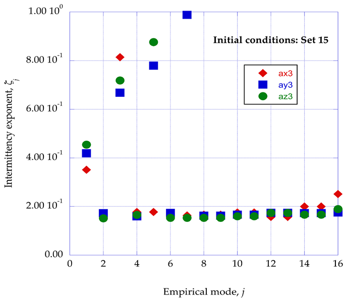
Figure 12. The intermittency exponents are shown for the spectral velocity components, ax3, ay3, and az3, for the initial conditions of Set 15 at the stream wise location of x = 0.120, the normalized vertical location of η = 3.00 and the span wise velocity of we = 0.080.
spectral velocity components to yield the average intermittency exponent for the entire Set 5 initial conditions. The resulting intermittency exponent will be designated as . The value of the average intermittency exponent for initial conditions Set 5 is found to be = 0.349.
Arimitsu and Arimitsu [33] found, in the analysis of quantum turbulent intermittency, a value of = 0.326, while Arimitsu, et al. [34] found by DNS analysis of this same quantum system a value of = 0.345. We may be able to gain a better understanding of the fundamental characteristics of systems with high values of intermittency exponents through a comparison of these two different systems.
The low-temperature quantum superfluid system studied in [33] [34] appears to have negligible mutual friction between the superfluid and the normal fluid components. Therefore, the level of irreversibilities produced in the system would be very low. In the three-dimensional boundary-layer with initial conditions given in Set 5 of Table 1, very low levels of instabilities are found in the nonlinear time-series solutions of the modified Lorenz equations. Subsequently, low values are predicted for the entropy generation rates for the initial conditions of Set 5. Thus, the similarity between these two systems is that they each have very low levels of irreversibilities.
However, when we move to the initial conditions Set 6, the first significant instability is found in the nonlinear time series solutions of the modified Lorenz equations. These instabilities give rise to a higher rate of dissipation of turbulent kinetic energy, thus increasing the irreversibilities in the process. This increase is reflected in the local peak in the entropy generation rate for Set 6, as indicated in Figure 3.
The computation of entropy generation rates reported here are for a three-dimensional laminar boundary layer located at a stream wise distance of 0.120 on a 1 m scale, with a stream wise velocity of unity, and at a normalized vertical distance in the boundary layer, η = 3.0, with the edge of the boundary layer at = 8.00, or 37.5 percent of the boundary-layer thickness. This location is approximately the position of the hot-wire measurements reported by Meneneau and Sreenivan [35] .
Table 2 shows the average intermittency exponents for a selected range of initial conditions, corresponding to the patterns apparent in Figure 3. Also shown are values of intermittency exponent used in a number of studies of the fractal nature of the dissipation of turbulent kinetic energy. The referenced values of the intermittency exponents are the values assumed in the indicated reference as either a given value for the analysis or an experimental value for comparison.
An overall average intermittency value was determined by averaging over Sets 6 - 10 and 14 - 16 with the results that = 0.241, which agrees with the universally accepted value of approximately 0.24 [33] [36] . It should also be noted that, in an analysis of the number of steps in the cascade process of the dissipation of turbulent kinetic energy [36] , the number of steps was found to be 16.4, which is close to the number of empirical modes, 16, that we have found from the power spectral density results.
6.5. Kinetic Energy Available for Dissipation
The source of the kinetic energy to be dissipated through the empirical modes is considered as the local steady-flow kinetic energy, u2/2, at the normalized vertical distance, η = 3.0 in the x-y plane boundary layer. This kinetic energy is assumed to be distributed over the three fluctuating velocity components. The fraction of kinetic energy in the x-direction velocity component is denoted as , the fraction of kinetic energy in the y-direction velocity component is denoted as and the fraction in the z-direction velocity component is denoted as . The fraction of dissipation kinetic energy within each empirical mode of the power spectral energy distribution is denoted as . Then the total rate of dissipation of the available fluctuating kinetic energy for the stream wise, normal and span wise velocity components is the summation, over the empirical modes, j, of the product of the kinetic energy fraction of each mode, , times the intermittency exponent for that mode, [3] .
The empirical intermittency exponent for each of the empirical modes has been obtained from the expression (Equation (16)) given by Arimitsu and Arimitsu [31] . Thus, values are available for the input energy source for the non-equilibrium ordered regions, the fraction of the fluctuation kinetic energy
Table 2. This table shows the average value for the intermittency exponents for a selected range of sets of initial conditions. Also shown are comparable values from selected references.
available in each of the empirical modes within the non-equilibrium ordered regions, and the fraction of the energy in each of the empirical modes that dissipates into background thermal energy, thus increasing the thermodynamic entropy. Concepts from non-equilibrium thermodynamics are used to calculate the dissipation process for the ordered regions as a general relaxation process. This is considered in the next section.
7. Entropy Generation Rates through the Dissipation of Ordered Regions
de Groot and Mazur (pp. 221-230 [37] ), from the concepts of non-equilibrium thermodynamics, write the equation for the entropy generation rate in an internal relaxation process as:
. (17)
Here, s is the entropy per unit mass, μ is the mechanical potential for the transport of the ordered regions in an external context and J(x) is the flux of kinetic energy through the ordered regions available for dissipation into thermal internal energy. The dissipation of the ordered regions into background thermal energy may be considered as a two-stage process from the transition of the ordered regions into equilibrium thermodynamic states and a turn-over process of the downstream velocity in the initial state to the final equilibrium state of the velocity over the internal distance x. The local boundary layer steady state velocity is written as , where is the derivative of the Falkner-Skan stream function f with respect to the normalized distance η. The expression for the entropy generation rate (in Joules/(m3∙K∙s)) through the non-equilibrium ordered regions is then written as [3] :
. (18)
In this expression, ρ is the density of the working substance, T is the temperature and ue is the free stream velocity. The dissipation rate for each of the three fluctuating spectral velocity components is included in Equation (18).
The kinetic energy in each spectral mode available for final dissipation into equilibrium internal energy is computed for each of the spectral peaks shown in Figure 7. The empirical entropy for each of the regions indicated by the spectral peaks is found from the singular value decomposition process applied to the given time series data segment. The connecting parameter, the empirical entropic index, is then extracted from the resulting value of the empirical entropy. The empirical entropic indices then allow the extraction of the corresponding intermittency exponents.
8. Discussion
There are two significant issues with the computational procedure and the results reported in this article. First, there have been no comparable computational results which would validate the procedures adopted here. Second, experimental validation is sparse and applies only to selected aspects of the computational approach and the results. However, the computational procedure is innovative in that it provides a method for the incorporation of a deterministic set of equations for the development of instabilities within the steady state environment of a three-dimensional laminar boundary layer flow. The results indicate that the entropy generation rates resulting from nonlinear interactions in a three-dimensional laminar boundary-layer flow are significantly affected by the particular initial conditions that are applied to the longitudinal vortex structure and the adjacent laminar boundary layer flow.
The counter clockwise rotating longitudinal vortex structure creates a viscous boundary layer along the z-y plane of the flow configuration. This viscous boundary layer is orthogonal to the laminar boundary layer in the x-y plane in the stream wise direction. It is shown that this nonlinear interaction creates instabilities within the three-dimensional flow configuration.
The computational results reported here for the entropy generation rates for a helium mixture boundary layer flow are obtained at the stream wise location of x = 0.120, in the range of stream wise locations from x = 0.06 to x = 0.18, for the normalized vertical station of η = 3.00. The weighting factor K in Equation (5) has been found to yield the prediction of instabilities for a value of K = 0.05. In an experimental investigation of laminar boundary layer receptivity to surface mass injection, Sengupta (pp. 158-170 [15] ) found that the coefficient of 0.05 for a time-dependent sinusoidal surface mass injection rate also initiated instabilities within a laminar boundary-layer flow. We thus have the implication that Equation (5) is a proper choice for the transformation of the Townsend equations for the fluctuating velocity components into a modified Lorenz format.
Free stream turbulence levels provide the turbulent kinetic energy that enters the wall shear layer. However, this level is attenuated within the layer and only a portion is available to serve as the initial conditions for the solution of the modified Lorenz equations describing the development of instabilities within the layer. Schmid and Henningson (pp. 430-436 [11] ) discuss the resulting formation of stream wise vortices, streaky structures, and the subsequence formation of turbulent spots through the interaction of this turbulence level within the wall boundary layer flow.
In the study reported here, we have modeled the interaction of a longitudinal vortex structure with a stream wise developing boundary layer through the time dependent modified Lorenz equations and have applied a range of initial conditions to the solutions of these equations.
Fluctuating spectral velocity components are found within the time-series solutions for the modified Lorenz equations. Statistical processing of the solutions indicates the presence of ordered regions embedded within the nonlinear time-series solutions. The dissipation of these ordered regions into equilibrium thermodynamic states yields the entropy generation rates for the three-dimensional interaction flow environment. Significant entropy generation rates are predicted for the specified sets of initial conditions applied to the solutions. The results for these entropy generation rates indicate a strong correlation of the entropy results with the levels of the applied initial conditions and that a pattern emerges as a function of the increasing levels of the initial condition equivalent turbulence intensities.
The sensitivity to initial conditions of the Lorenz format spectral velocity equations may provide a means of connecting the incorporation of these time dependent spectral equations in the computational procedure with the concept of bypass transition of the boundary layer flow due to outside disturbances.
9. Conclusions
The flow configuration of a longitudinal vortex structure and an adjacent laminar boundary layer for a helium mixture flow provides a three-dimensional nonlinear interaction of laminar boundary layers. In the study reported in this article, the velocity fluctuations produced by the instabilities that occur in such an interaction have been modeled through the transformation of the Townsend equations for the velocity fluctuations into a set of nonlinear deterministic Lorenz equations for the spectral velocity components of the fluctuations in the time frame.
The steady boundary-layer velocity profiles in the longitudinal-normal plane and the span wise-normal plane are computed using well-established numerical methods and serve as control parameters for the solutions of the modified Lorenz equations for the time-dependent spectral velocity components. It is shown that the solutions of the nonlinear deterministic modified Lorenz equations are strongly dependent on the values for the initial conditions applied to the solutions. Eighteen sets of initial conditions are examined for the resulting effects on the final values for the computed entropy generation rates.
Power spectral density analysis of the nonlinear time series indicates the presence of sixteen ordered spectral velocity modes within the time series data. Integration over each of these modes provides the ordered energy available within that mode for dissipation into background thermal energy, or increase of entropy. From the singular value decomposition of the time series data, the fraction of kinetic energy in each of the sixteen modes yields a corresponding value of empirical entropy for that mode. The value of empirical entropy yields the value for the Tsallis empirical entropic index, from which the corresponding intermittency exponent for each mode is obtained. Combining these results yields the expression of the total entropy generation rate for all of the ordered modes.
The entropy generation rates through the dissipation of these ordered regions are computed for eighteen sets of initial conditions for the given helium boundary layer flow environment. Strong correlation is found between the predicted entropy generation rates and the initial conditions applied for the solutions of the modified Lorenz equations, both in amplitudes of the generation rates and the emergent of significant patterns of the entropy generation rates as a function of the intensity levels of the applied initial conditions.
These results offer a deterministic path to the understanding of bypass transition and a foundation for the development of an understanding of the dynamics of turbulent spots in the transition from laminar to turbulent flows.
Conflicts of Interest
The author declares no conflict of interest.
Cite this paper
Isaacson, L.K. (2018) Entropy Generation through the Interaction of Laminar Boundary-Layer Flows: Sensitivity to Initial Conditions. Journal of Modern Physics, 9, 1660-1689. https://doi.org/10.4236/jmp.2018.98104
References
- 1. Townsend, A.A. (1976) The Structure of Turbulent Shear Flow. 2nd Edition, Cambridge University Press, Cambridge.
- 2. Sparrow, C. (1982) The Lorenz Equations: Bifurcations, Chaos, and Strange Attractors. Springer-Verlag, New York. https://doi.org/10.1007/978-1-4612-5767-7
- 3. Isaacson, L.K. (2017) Entropy, 19, 278. https://doi.org/10.3390/e19060278
- 4. Isaacson, L.K. (2016) Entropy, 18, 47. https://doi.org/10.3390/e18020047
- 5. Isaacson, L.K. (2016) Entropy, 18, 279. https://doi.org/10.3390/e18080279
- 6. Walsh, E.J. and Hernon, E. (2006) Entropy, 8, 25-30. https://doi.org/10.3390/e8010025
- 7. Hellberg, C.S. and Orszag, S.A. (1988) Physics of Fluids, 31, 6-8. https://doi.org/10.1063/1.867010
- 8. Singer, B.A. (1996) Physics of Fluids, 8, 509-521. https://doi.org/10.1063/1.868804
- 9. Ersoy, S. and Walker, J.D.A. (1985) Physics of Fluids, 28, 2687-2698. https://doi.org/10.1063/1.865226
- 10. Belotserkovskii, O.M. and Khlopkov, Y.I. (2010) Monte Carlo Methods in Mechanics of Fluid and Gas. World Scientific Publishing, Singapore, 101-102.
- 11. Schmid, P.J. and Henningson, D.S. (2001) Stability and Transition in Shear Flows. Springer-Verlag, New York, 401-465. https://doi.org/10.1007/978-1-4613-0185-1_9
- 12. Cebeci, T. and Bradshaw, P. (1977) Momentum Transfer in Boundary Layers. Hemisphere, Washington DC, 319-321.
- 13. Cebeci, T. and Cousteix, J. (2005) Modeling and Computation of Boundary-Layer Flows. Horizons Publishing, Long Beach.
- 14. Hansen, A.G. (1964) Similarity Analyses of Boundary Value Problems in Engineering. Prentice-Hall, Englewood Cliffs, 86-92.
- 15. Sengupta, T.K. (2012) Instabilities of Flows and Transition to Turbulence. CRC Press, Boca Raton, 171-200.
- 16. Attard, P. (2012) Non-Equilibrium Thermodynamics and Statistical Mechanics: Foundation and Applications. Oxford University Press, Oxford. https://doi.org/10.1093/acprof:oso/9780199662760.001.0001
- 17. Manneville, P. (1990) Dissipative Structures and Weak Turbulence. Academic Press, San Diego.
- 18. Isaacson, L.K. (2012) Entropy, 14, 131-160. https://doi.org/10.3390/e14020131
- 19. Pecora, L.M. and Carroll, T.L. (1996) Synchronization in Chaotic Systems. In: Kapitaniak, T., Ed., Controlling Chaos: Theoretical and Practical Methods in Nonlinear Dynamics, Academic Press Inc., San Diego, 142-145. https://doi.org/10.1016/B978-012396840-1/50040-0
- 20. Pérez, G. and Cerdeira, H.A. (1996) Extracting Messages Masked by Chaos. In: Kapitaniak, T., Ed., Controlling Chaos: Theoretical and Practical Methods in Nonlinear Dynamics, Academic Press Inc., San Diego, 157-160. https://doi.org/10.1016/B978-012396840-1/50043-6
- 21. Cuomo, K.M. and Oppenheim, A.V. (1996) Circuit Implementation of Synchronized Chaos with Applications to Communications. In: Kapitaniak, T., Ed., Controlling Chaos: Theoretical and Practical Methods in Nonlinear Dynamics, Academic Press Inc., San Diego, 153-156. https://doi.org/10.1016/B978-012396840-1/50042-4
- 22. Chen, C.H. (1982) Digital Waveform Processing and Recognition. CRC Press, Boca Raton, 131-158.
- 23. Press, W.H., Teukolsky, S.A., Vetterling, W.T. and Flannery, B.P. (1992) Numerical Recipes in C: The Art of Scientific Computing. 2nd Edition, Cambridge University Press, Cambridge.
- 24. Cover, T.M. and Thomas, J.A. (2006) Elements of Information Theory. 2nd Edition, John Wiley & Sons, Hoboken.
- 25. Holmes, P., Lumley, J.L., Berkooz, G. and Rowley, C.W. (2012) Turbulence, Coherent Structures, Dynamical Systems and Symmetry. 2nd Edition, Cambridge University Press, Cambridge. https://doi.org/10.1017/CBO9780511919701
- 26. Thomas, J.W. (1995) Numerical Partial Differential Equations: Finite Difference Methods. Springer-Verlag, New York. https://doi.org/10.1007/978-1-4899-7278-1
- 27. Isaacson, L.K. (2013) Entropy, 15, 4134-4158. https://doi.org/10.3390/e15104134
- 28. Rissanen, J. (2007) Information and Complexity in Statistical Modeling. Springer, New York.
- 29. Tsallis, C. (2009) Introduction to Nonextensive Statistical Mechanics. Springer, New York, 37-43. https://doi.org/10.1007/978-0-387-85359-8_3
- 30. Arimitsu, T. and Arimitsu, N. (2000) Physical Review E, 61, 3237-3240. https://doi.org/10.1103/PhysRevE.61.3237
- 31. Mandelbrot, B.B. (1983) The Fractal Geometry of Nature. W.H. Freeman and Company, New York, 97-105.
- 32. Frisch, U. and Parisi, G. (1985) Fully Developed Turbulence and Intermittency. In: Ghil, M., Benzi, R. and Parisi, G., Eds., Turbulence and Predictability in Geophysical Fluid Dynamics and Climate Dynamics, North-Holland, New York, 84-88.
- 33. Arimitsu, T. and Arimitsu, N. (2005) Journal of Physics: Conference Series, 7, 101-120. https://doi.org/10.1088/1742-6596/7/1/009
- 34. Arimitsu, T., Arimitsu, N. and Mouri, H. (2012) Physics of Fluid Dynamics, 4, 1-17.
- 35. Meneveau, C. and Sreenivasan, K.R. (1987) Nuclear Physics B, 2, 49-76. https://doi.org/10.1016/0920-5632(87)90008-9
- 36. Arimitsu, T. and Arimitsu, N. (2003) Condensed Matter Physics, 6, 85-92. https://doi.org/10.5488/CMP.6.1.85
- 37. De Groot, S.R. and Mazur, P. (1962) Non-Equilibrium Thermodynamics. North-Holland, Amsterdam.
Nomenclature
ai: Fluctuating i-th component of velocity wave vector
bn: Coefficient in modified Lorenz equations defined by Equation (9)
F: Time-dependent feedback factor
h: Integration time step (s)
j: Mode number empirical eigenvalue
J: Net source of kinetic energy dissipation rate, Equation (17)
k: Time-dependent wave number magnitude
ki: Fluctuating i-th wave number of Fourier expansion
K: Adjustable weighting factor
n: Stream wise station number
P: Local static pressure (N∙m−2)
qj: Empirical entropic index for the empirical entropy of mode, j
rn: Coefficient in modified Lorenz equations defined by Equation (8)
s: Entropy per unit mass (J∙kg−1∙K−1))
sn: Coefficient in modified Lorenz equations defined by Equation (8)
Sempj: Empirical entropy for empirical mode, j
: Entropy generation rate through kinetic energy dissipation (J∙m−3∙K-1∙s−1)
t: Time (s)
u: Mean stream wise velocity in the x-direction in Equation (4)
u’: Fluctuating stream wise velocity in Equation (4)
ue: Stream wise velocity at the outer edge of the x-y plane boundary layer
ui: The i-th component of the fluctuating velocity
Ui: Mean velocity in the i-th direction in the modified Lorenz equations
we: Span wise velocity at the outer edge of the z-y plane boundary layer
x: Stream wise distance
xi: i-th direction
xj: j-th direction
y: Normal distance
z: Span wise distance
Greek Letters
δ: Boundary layer thickness (m)
δlm: Kronecker delta
: Intermittency exponent for the j-th mode in Equation (18)
η: Transformed normal distance parameter
η¥: Transformed outer edge of the boundary layer
: Fraction of kinetic energy in the stream wise component
: Fraction of kinetic energy in the normal component
: Fraction of kinetic energy in the span wise component
λj: Eigenvalue for the empirical mode, j
μ: Mechanical potential in Equation (17)
v: Kinematic viscosity of the gas mixture (m2∙s-1)
: Kinetic energy in the j-th empirical mode
ρ: Density (kg∙m−3)
σy: Coefficient in modified Lorenz equations defined by Equation (7)
σx: Coefficient in modified Lorenz equations defined by Equation (7)
τw: Wall shear stress (N∙m−2)
Subscripts
e: Outer edge of the laminar boundary layer
i, j, l, m: Tensor indices
x: Component in the x-direction
y: Component in the y-direction
z: Component in the z-direction