Journal of Modern Physics
Vol. 4 No. 8A (2013) , Article ID: 36272 , 5 pages DOI:10.4236/jmp.2013.48A015
Inflation Playing by John Lagrangian
Faculté des Sciences et Techniques, Université d’Abomey-Calavi, Cotonou, Bénin
Email: kanfon@yahoo.fr, gastonedah@yahoo.fr, ezinvi.baloitcha@cipma.uac.bj
Copyright © 2013 Antonin Kanfon et al. This is an open access article distributed under the Creative Commons Attribution License, which permits unrestricted use, distribution, and reproduction in any medium, provided the original work is properly cited.
Received June 1, 2013; revised July 13, 2013; accepted August 9, 2013
Keywords: John Lagrangian; Inflation
ABSTRACT
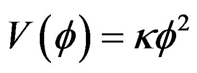
Our goal is to reproduce inflation through the coupling between the non-minimal first derivative of the scalar field and the Einstein tensor in which we introduced a potential. We analyse the inflation by examining the equation of state, the expansion parameter and the scale factor. We have shown that when the potential is proportional to the field  and proportional to the square of the field, inflation does not appear; but when the potential is an exponential function of the scalar field, this model brings up inflation. Inflation does not occur when the time t is near minus infinity but it is noticed a few units of Planck time.
1. Introduction
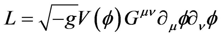
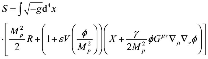
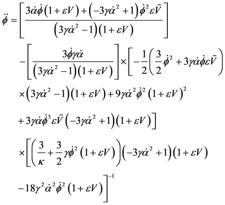
Based on observations [1-3], we can say that the universe today is almost flat. If this is the case, i.e., it has remained flat since the beginning of time? To this problem of flatness, we can add the horizon problem. To solve these problems Englert and Guth proposed in [1] primordial inflation. The universe would have grown exponentially just after the Big Bang. Many models of inflation exist and most involve a scalar field which undergoes a phase transition during inflation. Many of these models use a potential that needs to be adjusted so that the theory is consistent with the observations. In this paper, we develop models of inflation from non minimal coupling to gravity. The first scalar-tensor theories involving nonminimal couplings are known as coupling Brans-Dike [4]. This work is based on an article published in 1974 by [5] followed by [6] where they show that only four families of terms lead to a violation of the equivalence principle, while ensuring to obtain the equations of motion of the second member. These couplings are given in [6] as the “Fab Four”. In our work, we consider a Lagrangian with two parts: the first is the non-minimal derivative coupling of the form
 (1)
(1)
nicknamed John in Fab Four. The second part consists of a minimal coupling with a multiplicative potential [7]. In other words, we relied on the work of [4,8,9], but here we have a potential which multiplies the kinetic part of the Lagrangian.
After building the action, we deduced the different equations by considering a flat space. We then presented some cosmological models and which followed by a discussion of those models.
2. Mathematical Model
2.1. Action
Let 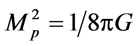 be the reduced Planck mass.
Let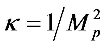 ,
, 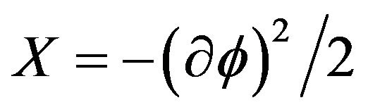
and
 (2)
(2)
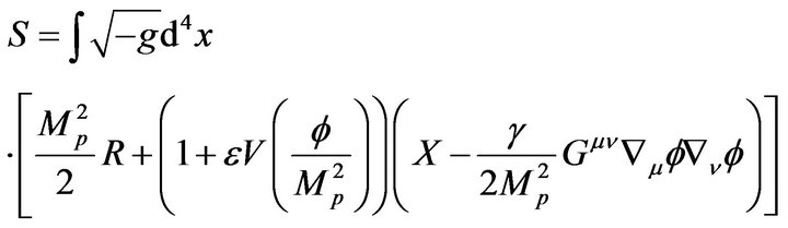
Which is equivalent to
 (3)
(3)
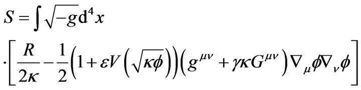
where ε and γ are constants dimensionless coupling; κ is 1/L2,  is 1/L. This action can be written
 (4)
(4)
ε = 0, we find the models studied by [8] and [4]
2.2. Equations of Motion
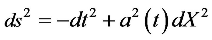
Consider a spatially-flat cosmological model with the metric
 (5)
(5)
With  the scale factor and
 ![]() the Euclidian metric. If one assume
the Euclidian metric. If one assume , then the cosmological equations which derive from the action (4) can be written
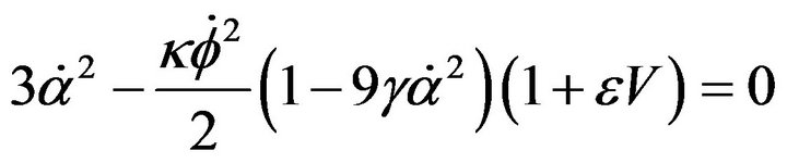 (6)
(6)
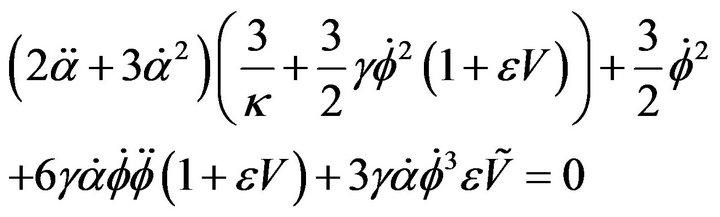 (7)
(7)
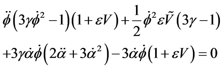 (8)
(8)
where
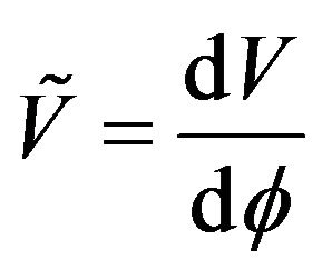
The Equations (6) and (7) are the equation of movement; 8 is the Klein-Gordon equation. If one poses
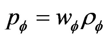
where  and
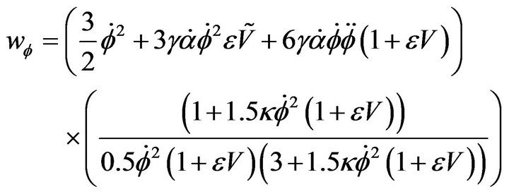
and  are respectively the pressure and the matter density of the field. We can use 6 and 7 to determine equation of state (EoS)
 (9)
(9)
3. Results and Discussion
Given the complexity of the equations, we did not obtain solutions analytics.
3.1. Decoupled Equations
Before starting the numerical solution, we will work Equations (7) and (8) to separate ![]() and
and 
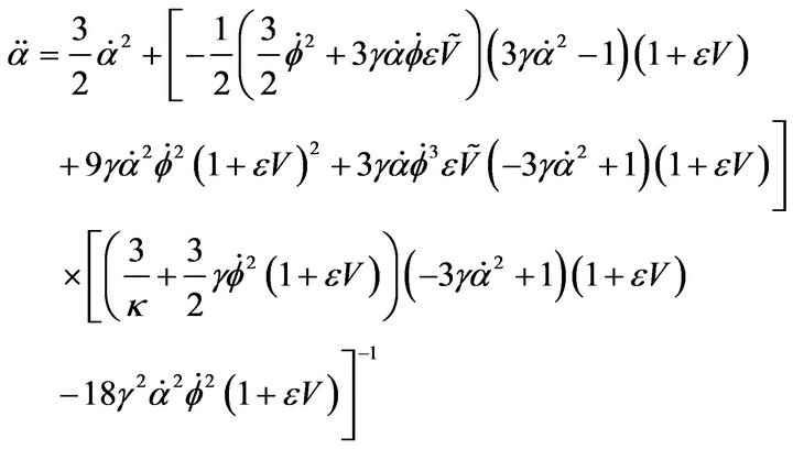 (10)
(10)
 (11)
(11)
We perform numerical integration by using matlab ode 45 precisely embedded Runge-Kutta method.

When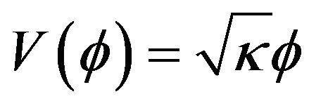 , the evolution of the state equation shows that with the presence of this potential, the field acts like the dark matter for ε negative or positive. The acceleration parameter goes to zero. The field ϕ vs the scale factor is a constant. This model does not accommodate inflation. These plots (Figures 1-4) have been obtained by numerical integration for an initial condition of φ = 10 in natural units in the case γ = 1.
Here also, the field starts with an EoS  but this field likes the dark matter with state equation equal 0; the acceleration parameter is negative; the Universe only decelerates as can been shown the four following plots (Figures 5-8)
We find that we can have cosmological models for only λ negative. We have shown the curves for . compared with those obtained for
  which is studied in the model [8]. The acceleration parameter (Figure 9) shows a universe initially accelerated after some time. So this time could correspond to the end of the inflationary epoch. Note that here, when ε is negative, universe deceleration makes less pronounced. Observing the curves α(t).
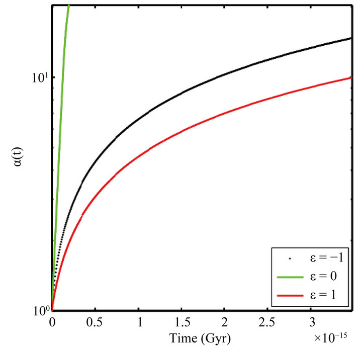
Figure 1. Evolution of α(t) for ε = −1, ε = 0 and ε = 1. As shown in the graph, when ε ≠ 0, α decreases quickly.
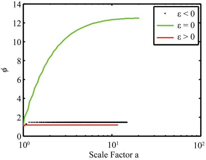
Figure 2. Evolution of the field Φ vs. the scale factor for ε = −1, ε = 0 and ε = 1. ε ≠ 0, ϕ is a constant.
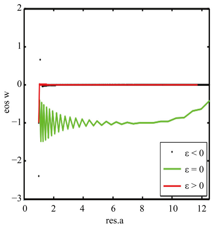
Figure 3. Evolution of the EoS wϕ vs. the scale factor (which is denoted by res.a) for ε = −1, ε = 0 and ε = 1. When ε = 0, the EoS wϕ starts at −1 and evolves by oscillation to 0. But when ε = 1, wϕ jumps vertically from −1 to 0 and no longer varies.
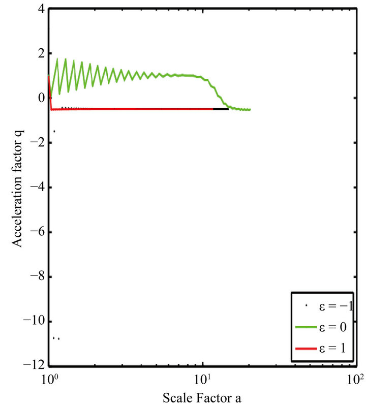
Figure 4. Evolution of the acceleration parameter q vs. the scale factor; ε = 0, this parameter remained positive long before the descent to 0. Against by ε ≠ 0, it drops abruptly to 0 and keeps this value.
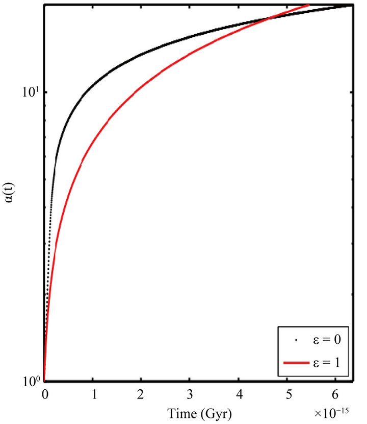
Figure 5. Evolution of α(t) for ε = 0 and ε = 1.
Figure 10 shows that these curves are linear at the origin, and this reinforces the notion of inflation at the origin of time. During this time the field  is an exponential function of the scale factor (Figure 11). During the inflationary epoch field behaved like a dark energy before undergoing a transition to the matter.
3.2. Discussion
We have presented above some numerical results ob-
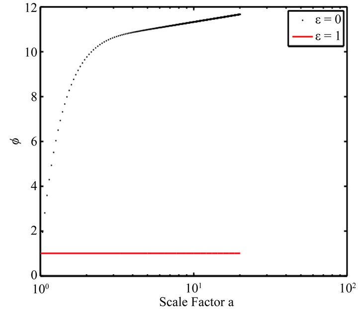
Figure 6. Evolution of the field ϕ vs. the scale factor for ε = −1, ε = 0 and ε ≠ 0, ϕ is a constant.
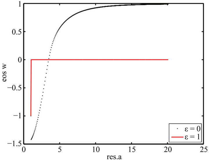
Figure 7. Evolution of the EoS wϕ vs. the scale factor for ε = 0 and ε = 1. ε = 0, the EoS wϕ starts at −1.5 and evolves to 1. But when ε = 1, wϕ jumps vertically from −1 to 0 and no longer varies.
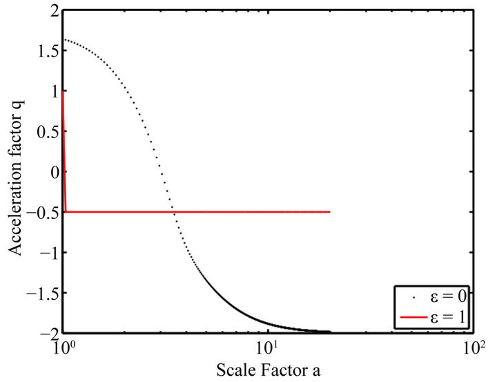
Figure 8. Evolution of the acceleration parameter q vs. the scale factor; ε = 0, this parameter remained positive long before the descent to −2. But ε ≠ 0, it drops abruptly to a negative value and keeps this value.
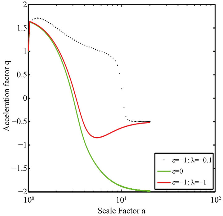
Figure 9. Evolution of the acceleration parameter q vs. the scale factor for (ε = −1, λ = −0.1), ε = 0 and (ε = −1, λ = −1). When (ε = 0).
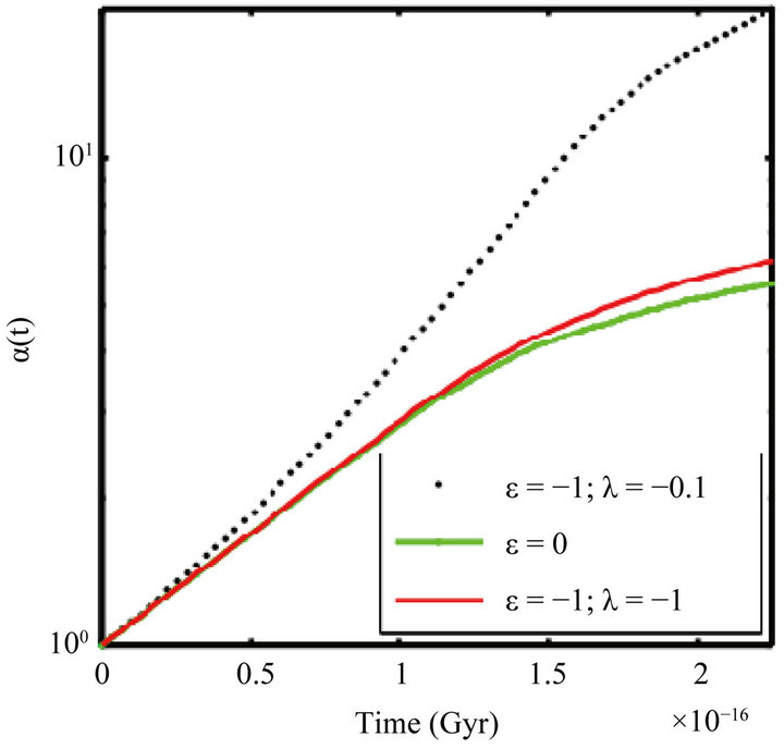
Figure 10. Evolution of α vs. the time for (ε = −1, λ = −0.1), ε = 0 and (ε = −1, λ = −1).
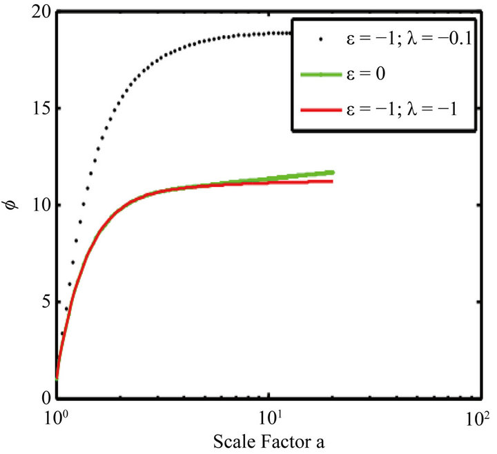
Figure 11. Evolution of the field ϕ vs. the scale factor for (ε = –1, λ = –0.1; ε = –0.1), and (ε = –1; λ = –1).
tained for some values of γ and ε from the equations of motion and the equation of state. This is α(t), the field , the parameters w and q as a function of the dynamic variable in cosmology, the scale factor a. Figures 1-4 show the behavior of these variables mentioned above for the potential
 . This is done for positive and negative values of ε which we compared the model john (ε = 0). Figure 3 shows that the equation of state w in the case of our model shows a sudden transition from Sitter universe
  to a universe dominated by dust
  for positive epsilon and in the same time, the acceleration parameter undergoes a dramatic drop from positive values to a negative constant. Is this a sign of the Big Bang? Curve α(t) in Figure 1 does not seem to confirm this thesis because the slope of this curve is linear for positive epsilon. Figures 5-8 show the behavior of the same magnitude as those shown in Figures 1-4, but with a potential proportional to the square of
  compared to the model without potential. We note that the results are similar to those obtained with a potential proportional to
 . In Figures 9-12, we have considered a potential V which is an exponential function of the field with negative λ. Figure 12 shows that equation of state is experiencing a phase transition from a regime to another Sitter regime before moving on to a universe dominated by matter when the model without potential evolved to a universe dominated by stiff matter. This means that the universe had to start inflation. The acceleration parameter (Figure 12) decreases from positive values to negative values, but this decrease is not as strong as in the model without potential, which is in agreement with the equation that after the double inflation, time a schema dominated by matter. The appearance of alpha confirms this thesis initially inflationary expansion followed by decelerated.
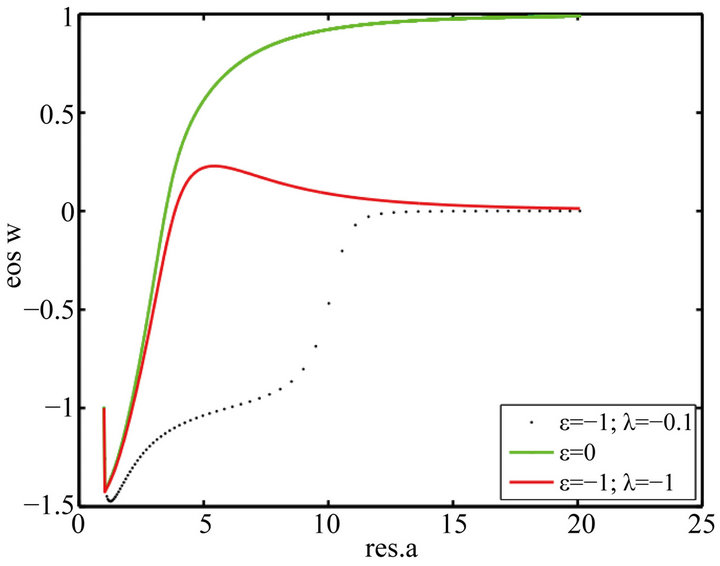
Figure 12. Evolution of the EoS wϕ vs. the scale factor for (ε = −1, λ = −0.1), ε = 0 and (ε = −1, λ = −1) When (ε = 0), the EoS wϕ starts at −1.5 and evolves to 1. But when ε = −1, wϕ evolves to 0.
4. Conclusions
We have shown that it is possible to obtain models of inflation by using the Fab Four. The model studied here is the model with potential multiplicative John. We limited the study to three types of potential: the potential that is proportional to the field , which is proportional to the square of
 , and the latter which produces inflation is a potential which is an exponential function of the field.
The results were compared to the John model without potential. Note that for this study, we imposed values to the parameters ε and γ and even λ. We were not able to perform a comprehensive study of these parameters.
On the other hand, we could consider a coupling between the scalar field and the fields that describe the matter, in which case the field transmits a part of its energy to matter.
REFERENCES
- C. Waelens and B. Craps, “Course of Introduction to Cosmology, KUL and VUB,” 2011.
- J. M. Alimi, A. Fuzfa, A. Boucher, V. Rasera, Y. Courtin and J. Corasaniti, Notices of the Royal Astronomical Society, 2010, pp. 775-790.
- M. P. Hobson, G. Efstathiou and A. N. Lasenby, “General Relativity, an Introduction for Physicists,” Cambridge University Press, Cambridge, 2006. doi:10.1017/CBO9780511790904
- J. P. Bruneton, M. Rinaldi, A. Kanfon, A. Hees, S. Schogel and A. Fuzfa, Advances in Astronomy, Vol. 2012, 2012, Article ID: 430694.
- G. W. Horndeski, International Journal of Theoretical Physics, Vol. 10, 1974, pp. 363-384. doi:10.1007/BF01807638
- C. Charmousis, E. J. Copeland, A. Padilla and P. M. Saffin, “General Second Order Scalar-Tensor Theory, Self Tunning, and the Fab Four,” 2011.
- A. Kanfon and D. Lambert, JMP, Vol. 3, 2012, pp. 1727- 1731.
- V. S. Sushkov, Physical Review D, Vol. 80, 2009, Article ID: 103505.
- E. N. Saridakis and S. V. Sushkov, Physical Review D, Vol. 81, 2010, Article ID: 083510.