Applied Mathematics
Vol.3 No.9(2012), Article ID:23014,3 pages DOI:10.4236/am.2012.39156
Local Influence Analysis of Generalized Linear Model
Basic Courses Department, Xuzhou Air Force College, Xuzhou, China
Email: wangshuling2007@yahoo.com.cn
Received May 6, 2012; revised July 30, 2012; accepted August 6, 2012
Keywords: Exponential Distributions; Local Influence Analysis; Influence Matrix
ABSTRACT
Nearly thirty years, the diagnosis and influence analysis of linear regression model has been fully developed. So far the local influence analysis of the generalized linear model has not yet seen in the literature. In this paper, local influence is discussed. Then, concise influence matrix is obtained. At last, an example is given to illustrate our results.
1. Introduction
Local influence analysis is proposed from the viewpoint of differential geometry [1]. Nearly thirty years, the diagnosis and influence analysis of linear regression model has been fully developed [2,3]. Regarding the generalized linear model, diagnosis has some results [4]. So far the local influence analysis of the generalized linear model has not yet seen in the literature, this paper attempts to study it.
2. Local Influence
Let  be an unknown k-dimensional parameter, whose domain is an open subset of Euclidean space
 .
.  is a object function(for example, likelihood function, punishment log-likelihood function).
  is a n-vector which denotes disturbed factor for example weightd or tiny shift. Let
  is the disturbed model, whose object function is
 .
.  is the estimate which is from
 .Given
  makes
makes  and
and
 , where
  has continuous second-order partial derivatives,
  is the function of
 . In geometry,
  denotes n-dimentional surface
 (1)
(1)
This image is called influence image, which vary with . The variation rate in
  of influence image reflects that the sensitivity of model where
  corresponds to the primary model. This method is called local influence [5]. Cook advanced that utilize influence curvature to measure the change of influence image near
 . Cook (1986) and Wei Bocheng (1990) pointed out that the influence curvature of
  is given by
 (2)
(2)
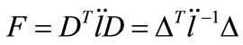
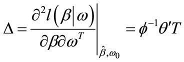
where  is the second derivatives of
  with respect to
 , and
, and
 (3)
(3)
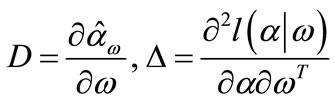
D and  is
is  matrix, where
 ,
, . The influence matrix is given by
 (4)
(4)
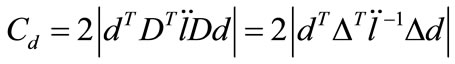
Formula (2.4) shows that the maximal influence curvature , where
  is the eigenvalue of
  whose absolute value is maximal, and
  is the corresponding eigenvector which is called the direction of maximal influence curvature. Escobar and Meeker (1992) pointed out that the diagonal value of influence matrix also is the important diagnostic statistics.
3. Local Influence Analysis of Model
Considering non-parametric regression model
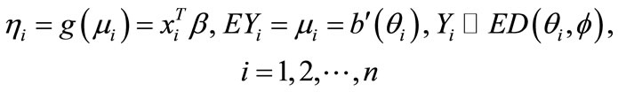 (1)
(1)
where  is the measure observations.
 ,
,  is i.i.d..
  denote that
  submit to exponential distributions, the corresponding density function is
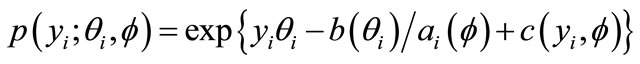 (2)
(2)
where ,
,  ,
,  and
and  are known functions,
  ,
, 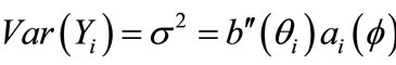 ,
,  and
and  are the first and second derivatives of
 ,
,  is p-dimension parameter,
  is the linear predict vector,
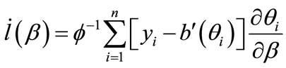
  is univariate increasing function. Let
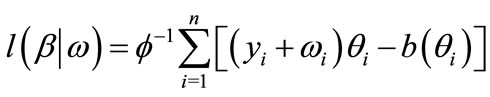
  is the log-likelihood function of
 .
.
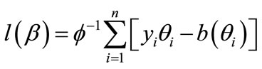 (3)
(3)
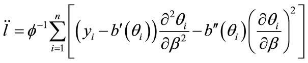
Let  and
and  are the first and second derivatives of
  with respect to
 , then
 (4)
(4)
 (5)
(5)
Supposed that the MLE of  in (3.1) is
 , and
, and  submits to

3.1. Weighted Perturbation Model
Suppose that ,
,  , then the weighted perturbation model can be shown that
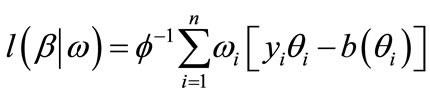 (3.1.1)
Substituting this result into (2.3) yields
 (3.1.2)
where ,
, . The second derivatives of
  with respect to
  is given by
 (3.1.3)
where  and
and .
.
Substituting (3.1.2) and (3.1.3) into (2.4), we obtain the corresponding influence matrix
 (3.1.4)
Here  denotes the direction of maximal influence curvature.
3.2. Response Variable Perturbation Model
Suppose that ,
,  , then the response variable perturbation model can be shown that
 (3.2.1)
Substituting this result into (2.3) yields
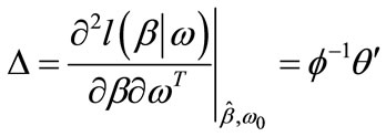 (3.2.2)
The second derivatives of  with respect to
  is given by
 (3.2.3)
Substituting (3.2.2) and (3.2.3) into (2.4), we obtain the corresponding influence matrix
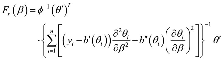 (3.2.4)
Here  denotes the direction of maximal influence curvature.
4. An Illustrative Example
(Kyphosis Data) Now we consider an example as the illustration for the above results. Considering a kyphosis data (see [6]). There are 81 patients who have been treated with chiropractic. There are four variables: kyphosis, Age, Number and Start. Wang xiaoming (2005) ultized a linear semi-parametric model to fit this test data. The regression analysis of kyphosis data are as follows (Table 1).
The local influence analysis results of kyphosis data are as follows (from Figures 1-3).
Figures 1 and 2 show that the sixth, forty-third, fifty-third and the eightieth data are influential points, Figure 3 shows that the first, second, third and fourth data are influential points. Actually, the direction of maximal influence curvature  also shows that the first, second,

Table 1. The regression analysis of kyphosis data.

Figure 1. The diagonal value of influence matrix Fω.
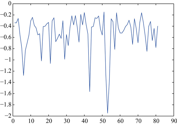
Figure 2. The diagonal value of influence matrix Fr.
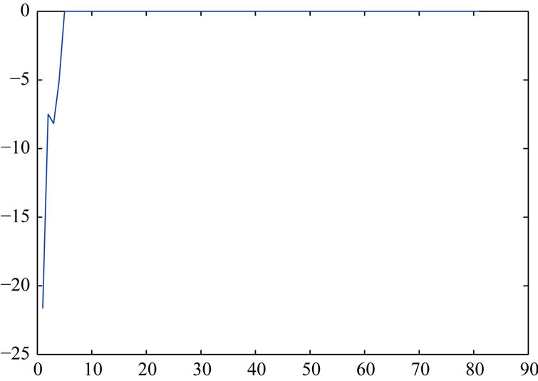
Figure 3. The direction of maximal influence curvature dω.
third and fourth data are influential points. This also proves that the above method is effective.
REFERENCES
- R. D. Cook, “Assessment of Local Influence (with Discussion),” Journal of the Royal Statistical Society (Series B), Vol. 48, 1986, pp. 133-169.
- R. D. Cook and S. Weisberg, “Residuals and Influence in Regression,” Chapman and Hall, New York, 1982.
- B. C. Wei, G. B. Lu and J. Q. Shi, “Statistical Diagnostics,” Publishing House of Southeast University, Nanjing, 1990.
- Y. Zhou, “Diagnostic and Numerical Example Analysis for Generalized Linear Model,” Journal of Sichuan University (Natural Science Edition), Vol. 44, 2007, pp. 1163- 1168.
- L. A. Escobar and W. Q. Meeker, “Assessing Influence in Regression Analysis with Censored Data,” Biometrics, Vol. 48, No. 2, 1992, pp. 507-528. HUdoi:10.2307/2532306U
- X. M. Wang and X. L. Han, “The Course of S-plus Applied Statistics,” Publishing House of Shanghai University of Finance and Economics, Shanghai, 2005.