Modern Economy
Vol. 3 No. 2 (2012) , Article ID: 18157 , 8 pages DOI:10.4236/me.2012.32033
Are Thai Manufacturing Exports and Imports of Capital Goods Related?
School of Development Economics, National Institute of Development Administration, Bangkok, Thailand
Email: komain_j@hotmail.com
Received November 8, 2011; revised January 5, 2012; accepted January 20, 2012
Keywords: Manufacturing Exports; Imports of Capital Goods; Economic Growth; Cointegration; Causality
ABSTRACT
This paper examines the relationship between manufacturing exports and imports of capital goods in Thailand using monthly data from January 2000 to July 2011. The results from bounds testing for cointegration show that there exists long-run equilibrium relationship between exports and imports of capital goods in manufacturing sector. In addition, the positive relationship between the growth rate of imports of capital goods and the growth rate of manufacturing exports is observed. The results support the notion that foreign capital is essential in the process of industrialization, and thus economic growth. A decline in imports of capital goods will reduce manufacturing exports and impedes economic growth in the future. It is also likely that exports of manufactured products are the main source of foreign exchanges to finance imports of capital goods which cannot be produced in the country due to comparative disadvantage.
1. Introduction
The long-run effect of capital accumulation on economic growth has been widely recognized in the economic development literature. Countries that reach high level of economic development seem to have higher equipment investment rates [1]. However, most of the world capital goods are produced in a small number of research and development (R & D)-intensive countries, while the rest of the world generally imports its capital equipment. Imports of capital goods by developing countries can be the key carriers of international spillovers from developed countries. Nevertheless, barriers to trade in capital equipment cause differences in productivity among countries [2]. Most of developing countries rely on imports of capital goods, which can boost national productive capacity by increasing total factor productivity, drive structural changes and increase competitiveness in the world market [3]. In addition, the quality of imported capital stocks differs with its composition, and thus the overall contribution to growth is different across countries [4]. In the international trade and trade policy literature, an open economy can benefit from importing foreign inputs in that they are important determinant of the link between trade and growth. The crucial role of international trade is to stimulate growth by providing a wider range of intermediate inputs, which in turn facilitates more R & D or learning by doing activities [5]. The contrary view is that trade can have a negative impact on growth of one trading partner, which is usually the less developed country (LDC). For LDCs, trade with developed countries can be harmful to their industrialization, and thus makes poor countries remain poor [6].
Development economists also recognize that foreign capital and inputs are essential in the process of industrialization, and thus economic growth. According to [7], a decrease in imports of capital goods will reduce the growth rate. Using cross-sectional data of countries for the period 1960-1985, [8] finds that the ratio of imports in investment or the ratio of imported to domesticcally-produced capital goods has significantly positive effects on per capita income growth rate across countries, but the share of total imports in GDP has no role in growth. The empirical results are consistent with the notion that imported capital goods have a higher productiveity than domestically-produced capital goods. Similar finding using panel data is that investment in domesticcally produced equipment reduces the growth rate while investment in imported equipment increases it [9]. On the contrary, [10] employs and augmented Solow model to control for the roles of human capital and labor force growth and finds an evidence showing that returns to equipment investment are very high in developing countries. Furthermore, it can be argued that developing countries that have a comparative disadvantage in machinery production, but a comparative advantage in consumer goods production, can benefit from trade in terms of growth through the importation of cheaper and better machinery. Some economists also emphasize the role of human capital, for example [11] finds a negative relationship between imports of capital goods and growth for countries with lowest level of human capital. The positive relationship is minimal in countries with low level of human capital. For countries without the resources to take advantage of the embodied advanced technology, investing in imported capital good can be unproductive.
Most of capital goods (machinery and equipment) operated in developing Asian countries, including Thailand, are imported. Imported capital goods enhance technological capability through exports of high value-added goods that requires modern technology [12]. The statistics showing technological readiness index scores of selected Asia-Pacific countries from 2008 to 2009 indicate that Thailand ranked ninth with the index score of 3.37, while Singapore had the highest index score [3]. In the late 1970s, Thailand switched from the import-substitution to exported-oriented policy. The intensive export promotion began in the early 1980s. The high economic growth rates were observed in the late 1980s until the 1997 financial crisis. Trade policy with tariff reduction has induced imports of machinery along with raw materials and semi-finished products. The share of manufacturing exports in total exports accounted for almost 90 percent during 1993 to 2008. The export-led growth hypothesis is valid for Thailand [13]. The long-run relationship between to total exports and quarterly GDP exists. This relationship is the same using only manufacturing exports.
In this study, the role of manufacturing exports on growth is not the main focus, but rather examines the relationship between manufacturing exports and imports of capital goods during January 2000 and July 2011.1 The real effective exchange rate is also included in the cointegrating equation to examine the impact of this variable on manufacturing exports and imports of capital goods. Furthermore, movements in real effective exchange rate could capture the impact of the 2007 subprime crisis in the United States on the Thai economy. The reason is that a swing in the exchange rate could be caused by the subprime crisis and would in turn affect exports and imports. The ARDL-ECM model, also known as “bounds testing for cointegration”, proposed by [14] is used to analyze the level relationship among manufacturing exports, imports of capital goods and real effective exchange rate.2 The advantage of this procedure is that it does not require that all variables be integrated of order one (or be I(1) series) as required by other tests of cointegration. The bounds testing for coinegration can be used even though variables are integrated of order zero or order one, or mutually cointegrated. The results show that there is a long-run relationship between manufacturing imports, imports of capital goods, and real effective exchange rate. In addition, there is a short-run relationship between the growth rate of manufacturing exports and the growth rate of imported capital goods. The paper is organized as follows. Section 2 describes the data and the methods of estimation. Section 3 presents empirical results. The last section gives conclusion with policy implication.
2. Data and Methodology
2.1. Data
In order to test the cointegration of variables, the monthly data of manufacturing production, manufacturing exports, imports of capital goods, and real effective exchange rate are retrieved from the Bank of Thailand during January 2000 and July 2011. All series are in the quantity indexes, except for real effective exchange rate, which is the index of weighted average of foreign currencies per domestic currency (Thai baht). The sample size is 139 month. All series are seasonally adjusted by the author.
2.2. Cointegration Tests
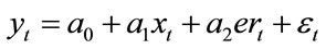
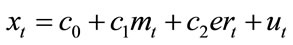
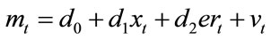
The multivariate cointegration test with three variables in each equation is adopted to determine the short-run and long-run relationship among variables. The following long-run equations are specified as:
 (1)
(1)
 (2)
(2)
 (3)
(3)
and
 (4)
(4)
where y is the log of manufacturing production index, x is the log of manufacturing exports index, m is the log of imports of capital goods index, and er is the log of real effective exchange rate index. The above equations can be estimated by the ordinary least square (OLS) method.
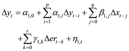
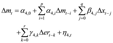
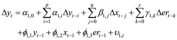
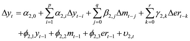
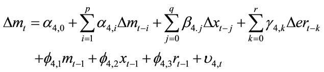
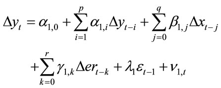
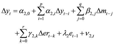
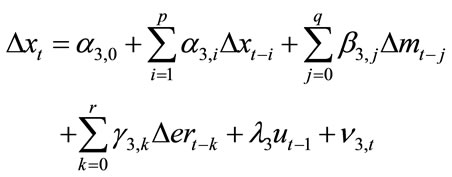
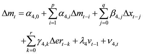
A conditional autoregressive distributed lag (ARDL) and error correction mechanism (ECM) proposed by [14] can be used to test for cointegration of variables in all four equations. The ARDL models are specified as
 (5)
(5)
 (6)
(6)
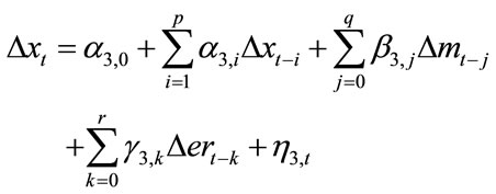 (7)
(7)
 (8)
(8)
where p, q, and r are the optimal number of lagged differences of the three-variable ARDL models. The grid search method can be used for selecting p, q, and r from the most parsimonious ARDL(p, q, r) model. By adding the appropriate lagged level variables into Equations (5)- (8), the computed F-statistics are obtained by estimateing the following equations.
 (9)
(9)
 (10)
(10)
 (11)
(11)
 (12)
(12)
To examine whether cointegration exists, one can use the computed F-statistic to compare with the critical values of [14]. If the computed F-statistic is above the upper bound critical value, the null hypothesis of no cointegration is rejected. When the computed F-statistic is below the lower bound critical value, the null hypothesis is accepted. The computed F-statistic taking the value between the upper and low bound critical value indicates that the result is inconclusive. If cointegration exists, replacing the lagged level variables in each equation with the one-period lagged error term from the estimated long-run equation will yield the coefficient of the error correction term.
2.3. Short-Run Dynamics
When cointegration exists, the ECM model can explain adjustment toward long-run equilibrium. The ECM models can be specified as follows.
 (13)
(13)
 (14)
(14)
 (15)
(15)
 (16)
(16)
The significance of the estimated coefficient of the err correction term is important in that it shows the speed of adjustment toward the long-run equilibrium and the existence of long-run causality. When cointegration does not exist, the standard Granger causality test proposed by [18] can be performed on stationary series, either level or first difference stationary. Without the error correction term, the orders p, q, and r should be equal and the criteon for choosing the optimal lag length is Akaike Infortion Criterion (AIC). The Equations (13)-(16), will be reduced to one-directional causality test.
3. Empirical Results
3.1. Results of Unit Root Tests
Before performing cointegration tests, the wo popular unit root tests, Augmented Dickey-Fuller (ADF) test proposed by [19] and Phillips and Perron (PP) test prosed by [20] are employed. The results of unit root tests are reported in Table 1.
The ADF and PP tests with a constant only and a conant and a trend are used to determine the stationarity property of each series. All tests indicate that the log of manufacturing output (x) and the log of real effective exchange rate (er) are integrated of order one, i.e., they are I(1) series. However, the PP test with a constant and a trend indicate that the log of exports (x) and the log of imports of capital goods (m) are statationary in the levels
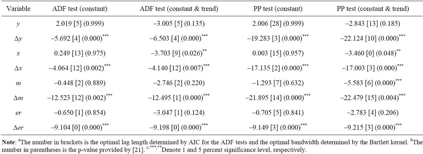
Table 1. Unit root tests results.
or integrated of order(0), I(0), while the other tests indite that both of them are I(1) series. Therefore it can be concluded the data show the complex nature of the time series property. Even though the ARDL bounds testing for cointegration does not require unit root tests, the relts show that the series might be mixed between I(0) and I(1). In addition, the maximum order of integration of all series does not exceed one as required by this method of cointegration test.
3.2. Results from ARDL Bounds Testing for Cointegration
Alternative cointegration tests such as [22,23] tests are not used because all series are not I(1) as required by both tests. Instead, the ARDL bounds testing for cointegration is suitable to use, and the procedure consists of three steps: 1) Estimating OLS regression with the first difference of the variables in Equations (5)-(8); 2) adding lagged-level variables and conducting the variable addition test specified in Equations (9)-(12), and 3) obtaining the computed F-statistics from step 2, and then compare them with the bound critical values that have two asymptotic critical values. The lower bound critical value assumes that the series are I(0) while the upper bound critical value assumes that they are I(1).
The lag length is chosen by the grid search method. With the small sample size of 139 observations, the search starts from the lowest number of lags and find the ARDL model that is free of serial correlation. Equations (5)-(8) have the ARDL (2, 1, 0), ARDL (2, 1, 0), ARDL (2,0,0), and ARDL(2,1,0) respectively. The estimates of Equations (9)-(12) are reported in Table 2.
The chi-square statistics in Table 2 test the null hypothesis that there is no serial correlation in the residuals of each estimated equation. This is a necessary condition for the bounds testing for cointegration. The results show that the null hypothesis is accepted in each equation. Since the ARDL model excludes the one-period lagged variables, adding the one-period lagged level of the three variables to the ARDL models yields the computed Fstatistics reported in Table 3.
In Table 3, no cointegration is found for the output and manufacturing exports (Panel A), and output with imports of capital goods (Panel B) because the computed F-statistics of 1.490 and 1.503 are below the lower bound critical value of 3.17 at the 10 percent level of signifycance. The computed F-statistic for the exports and the imports of capital good equations (Panels C and D) are 5.672 and 11.040 respectively, and are above the upper bound critical value of 4.85 at the 5 percent level of significance. There for the null hypothesis of no cointegration is rejected. Thus it can be concluded that there is long-run relationship between manufacturing exports and imports of capital goods.3 Since no cointegrating relation is found for the estimates of Panels A and B in Table 2, Granger causality test is performed on first, differences of variables.4 The null hypothesis that the growth rate of manufacturing exports does not cause the growth rate of manufacturing output is accepted [F-statistic is 1.853 (p = 0.123)]. However, the null hypothesis that the growth rate of imported capital goods does not cause the growth rate of manufacturing output is rejected at the 5 percent level of significance [F-statistic is 6.415 (p = 0.012)]. Therefore, it can be claimed that an increase in imports of foreign capital enhances manufacturing output growth. This is consistent with the notion that foreign capitals are essential in the process of industrialization.
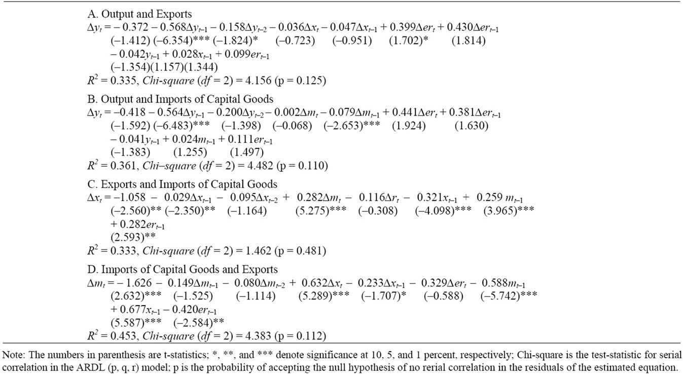
Table 2. Results from bounds testing for cointegration.
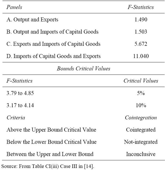
Table 3. Computed F-statistics.
3.3. Results of Long-Run Relationship between Exports and Imports of Capital Goods
The long-run relationship between manufacturing exports, imports of capital goods and real effective exchange rate is shown in Panel A of Table 4, while the long-run relationship between imports of capital goods, exports and real effective exchange rate is in Panel B.
In Panel A of Table 4, a one-percent increase in im-
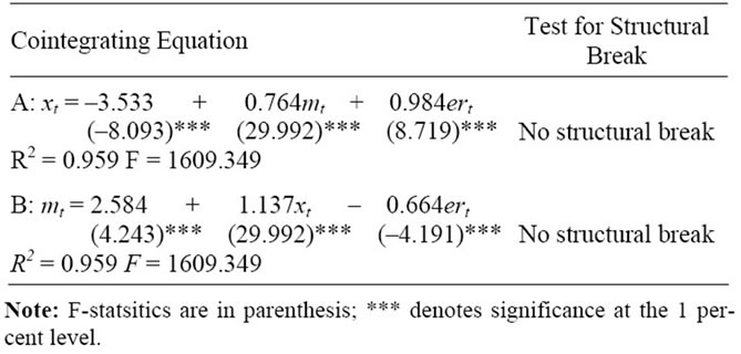
Table 4. Long-run relationship between exports and imports of capital goods.
ports of capital goods causes manufacturing exports to increase by 0.764 percent. A rise in real effective exchange rate (or real depreciation of domestic currency) cause manufacturing exports to increase by 0.984 percent. In Panel B of the table, a one-percent increase in manufacturing exports causes the imports of capital goods to rise by 1.137 percent. The impact of real exchange rate on imports and exports are consistent with the generalized condition in the international trade theory. A onepercent increase in real effective exchange rate causes imports of capital goods to fall by 0.664 percent and exports of manufactured products to rise by 0.764 percent.
The long-run equation should be stable when cointegration exists. Stability of the cointegrating relation is tested using CUSUM of squares and the results are shown in Figures 1 and 2.
There seem to be no structural breaks in both cointegrating equations since the line is in the band in both
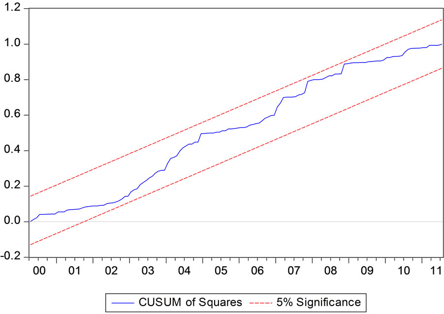
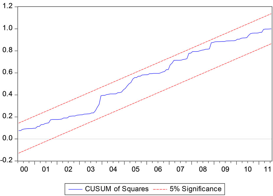
cases.
3.4. Results of Short-Run Dynamics
The error correction mechanism (ECM) models are estimated by adding the appropriate error correction term to the ARDL specified in Equations (15) and (16). The error correction terms (ECT) are the one-period lagged residuals (or error terms) of the cointegrating equations. The results of the estimated ECM models showing shortrun dynamics are reported in Table 5.
Since the ARDL models are free of autocorrelation, the estimated ECM models are also free of autocorrelation. The ARCH LM test shows not autoregressive heteroskedasticity in both Panels A and B of Table 5. In addition, the null hypothesis of normality in the residuals cannot be rejected. The results seem to support the adequacy of the estimated ECM models. The estimated coefficients of the one-period lagged error terms (ut-1 and vt-1) are between 0 and –1, and highly statistically significant in both estimated equations, i.e., –0.317 and –0.588. These results also confirm the existence of long-run equilibrium relationship among variables included in the two equations. Any deviation from long-run equilibrium will be corrected. In Granger causality sense, there exists long-run causality running from imports of
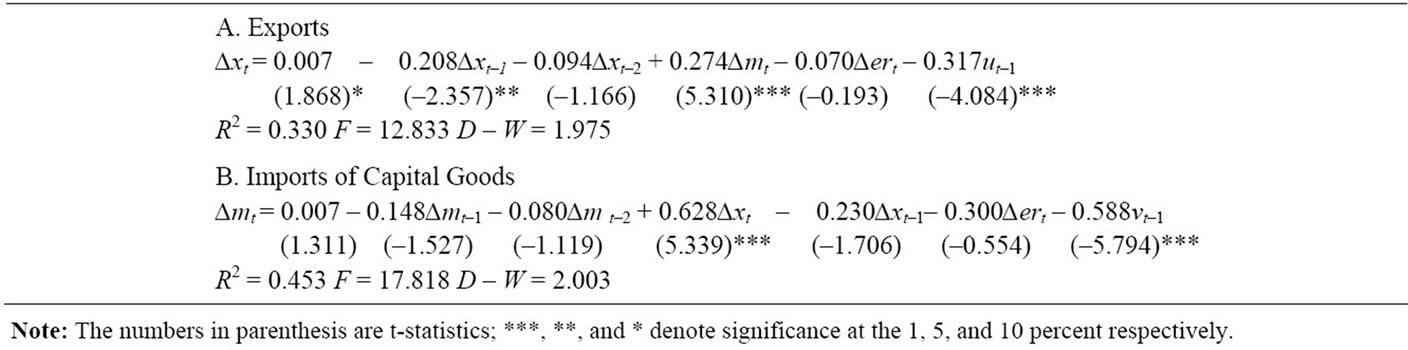
Table 5. Results of short-run dynamics.
capital goods and real effective exchange rate to manufacturing exports. Similarly, there also exists long-run causality running from manufacturing exports and real effective exchange rate to imports of capital goods. For short-run relationship, there is significantly positive relation between the growth rate of manufacturing exports and the growth rate of imports of capital goods with the coefficients of 0.274 and 0.628 in Panels A and B respectively. However, the change in real effective exchange rate plays no role in the short run.
The results from the present study show that there is significant long-run relationship between manufactured exports and imports of capital goods. In the short-run, the growth rate of manufactured exports and the growth rate of imports of capital goods are strongly related. Whether the structure of tariffs should be changed needs further research works. Policymakers might have implemented sufficient measures to stimulate manufacturing growth. According to [24], there is causality between skill-bias (caused by protection) and productivity growth. Adequate skill-intensive target can enhance growth, not only in the targeted sector, but also in other sectors. Thailand might need skill upgrading target that will benefit manufacturing firms.
4. Conclusions
Bounds testing for cointegration can be used to test the level relationship between variables and does not require unit root tests. However, the complex nature of the property of time series can be known using the popular ADF and PP tests. The justification for employing the bounds test is that all variables are not exactly I(1) series. The critical values provided are for the mixed between I(0) and I(1) series. If any variable is second order difference stationary or I(2) series, the procedure should not be valid. The results from cointegration test show that exports of manufactured products and imports of capital goods are cointegrated or have a long-run relationship. The impact of real effective exchange rate on manufacturing exports is positive while that the impact real effecttive exchange rate on imports of capital goods is negative. The traditional QSUM of square test is adopted, and the results show that the estimated cointegrating equations are stable. Additionally, the ECM model for an analysis of the short-run dynamics gives the significant coefficient of the error correction term, which implies that there exists long-run causality between variables in the specified model. The short-run relationship between the growth rate of manufacturing exports and that of imports of capital goods is positive. This indicates the interdependency of these two variables. Since coinintegration between manufacturing output and exports as well as output and imports of capital goods is not found. The standard Granger causality test is performed on first differences of variables. The causality test results show that the growth rate of manufacturing output does not depend on the growth rate of manufacturing exports, but depends on the growth rate of imports of capital goods.
Since an increase in imported capital goods Granger causes manufacturing production and manufacturing exports. The results are consistent with the notion that foreign capitals are essential in the industrialization process, and thus economic growth. The policy implication is that Thailand cannot reduce the imports of capital goods. Otherwise, manufacturing output and exports will decrease, which in turn can harm the overall growth rate. However, further research should emphasize the impact of imported capitals on total factor productivity growth using long-span annual data.
5. Acknowledgements
The author would like to thank anonymous referees for comments and suggestions.
REFERENCES
- J. B. De Long and L. H. Summers, “Equipment Investment and Economic Growth,” Quarterly Journal of Economics, Vol. 106, No. 2, 1991, pp. 445-502. doi:10.2307/2937944
- J. Eaton and S. Kortum, “Trade in Capital Goods,” European Economic Review, Vol. 45, No. 1, 2001, pp. 1195- 1235. doi:10.1016/S0014-2921(00)00103-3
- World Economic Forum, “The Global Competitiveness Reports, 2008-2009,” Geneva, 2008.
- F. Caselli and D. Wilson, “Importing Technology,” Journal of Monetary Economics, Vol. 51, No. 1, 2004, pp. 1-32. doi:10.1016/j.jmoneco.2003.07.004
- D. Quah and J. Rauch, “Openness and the Role of Economic Growth,” Mimeo, MIT, Cambridge, 1990.
- P. Krugman, “Trade, Accumulation, and Uneven Development,” Journal of Development Economics, Vol. 8, No. 2, 1981, pp. 149-161. doi:10.1016/0304-3878(81)90026-2
- A. Kruger, “The Effects of Trade Strategies on Growth,” Finance and Development, Vol. 20, No. 2, 1983, pp. 6-8.
- J. W. Lee, “Capital Goods Imports and Long-Run Growth,” NBER Working Paper, No. 4725, 1994.
- J. Mazumdar, “Imported Machinery and Growth in LDCs,” Journal of Development Economics, Vol. 65, No. 1, 2001, pp. 209-224. doi:10.1016/S0304-3878(01)00134-1
- J. Temple, “Equipment Investment and the Solow Growth Model,” Oxford Economic Papers, Vol. 50, No. 1, 1998, pp. 39-62.
- U. Dulleck and N. Foster, “Imported Equipment, Human Capital and Economic Growth in Developing Countries,” Working Paper No. 16, National Center for Economic Research, 2007.
- T. Tambunan, “Why Do Least Developed Countries in Asia Not Benefit from Transfers of Technology,” ARTNeT Policy Brief, No. 18, 2009.
- K Jiranyakul, “Recent Evidence of the Validity of the Export-Led Growth Hypothesis for Thailand,” Economics Bulletin, Vol. 30, No. 3, 2010, pp. 2151-2159.
- M. H. Pesaran, Y. Shin and R. I. Smith, “Bounds Testing Approaches to the Analysis of Level Relationship,” Journal of Applied Econometrics, Vol. 16, No. 3, 2001, pp. 289- 326. doi:10.1002/jae.616
- A. C. Arize and C. Augustine, “Imports and Exports in 50 Countries: Test of Cointegration and Structural Breaks,” International Review of Economics and Finance, Vol. 11, No. 1, 2002, pp. 101-105. doi:10.1016/S1059-0560(01)00101-0
- M. Irandoust and J. Ericson, “Are Exports and Imports Cointegrated? An International Comparison,” Metroeconomica, Vol. 55, No.1, 2004, pp. 49-64. doi:10.1111/j.0026-1386.2004.00182.x
- F. Sekman and S. Saribas, “Cointegration and Causality among Exchange Rate, Export and Import: Empirical Evidence from Turkey,” Applied Econometrics and International Development, Vol. 7, No. 2, 2007, pp. 71-78.
- C. W. J. Granger, “Investigating Causal Relations by Econometric Models and Cross-Spectral Methods,” Econometrica, Vo. 37, 1969, pp. 424-438. doi:10.2307/1912791
- D. A. Dickey and W. A. Fuller, “Likelihood Ratio Statistics and Autoregressive Time Series with a Unit Root,” Econometrica, Vol. 49, No. 4, 1981, pp. 1057-1072. doi:10.2307/1912517
- P. C. B. Phillips and P. Perron, “Testing for a Unit Root in Time Series Regression,” Biometrika, Vol. 45, No. 2, 1988, pp. 335-346. doi:10.1093/biomet/75.2.335
- J. G. MacKinnon, “Numerical Distribution Functions for Unit Root and Cointegration Tests,” Journal of Applied Econometrics, Vol. 11, No. 6, 1996, pp. 601-618. doi:10.1002/(SICI)1099-1255(199611)11:6<601::AID-JAE417>3.0.CO;2-T
- R. F. Engle and C. W. J. Granger, “Co-Integration and Error Correction: Representation, Estimation and Testing,” Econometrica, Vol. 55, No. 2, 1987, pp. 251-276. doi:10.2307/1913236
- S. Johansen, “Estimation and Hypothesis Testing for Cointegration Vectors in Gaussian Vector Autoregressive Models,” Econometrica, Vol. 59, No. 6, 1991, pp. 1551- 1580. doi:10.2307/2938278
- N. Nunn and D. Trefler, “The Structures of Tariffs and Long-term Growth,” American Economic Journal: Macroeconomics, Vol. 2, No. 4, 2010, pp. 158-194. doi:10.1257/mac.2.4.158
NOTES
1This period is quite restricted due to the availability of the monthly data. Also, it is the period after the turmoil from the 1997 Asian financial crisis.
2Many studies employ this procedure to examine the relationship between total exports and total imports, see [15-17] for example. However, these studies shed light on how countries face trade deficits or surpluses.
3Even though there is no long-run relationship between manufacturing output and manufacturing exports, and manufacturing output and import of capital goods, but imports of capital goods positively affect manufacturing exports. The empirical evidence from [13] who uses quarterly data during 1993 and 2008 shows that manufacturing exports positively affect real GDP of the country.
4The optimal lag for y, x, and er is 4 and for y, m, and er is one, which is determined by AIC.