World Journal of Condensed Matter Physics
Vol. 2 No. 4 (2012) , Article ID: 25050 , 11 pages DOI:10.4236/wjcmp.2012.24042
Effect of the Variable B-Field on the Dynamic of a Central Electron Spin Coupled to an Anti-Ferromagnetic Qubit Bath
![]()
1Department of Physics, Laboratory of Mesoscopic and Multilayer Structures, University of Dschang, Dschang, Cameroon; 2Department of Physics, Faculty of Sciences and Technics, University of Abomey-Calavi, Cotonou, Benin; 3Department of Thermal Engineering and Energetics, Douala University Institute of Technology, Douala, Cameroun; 4Department of Mechanical Engineering, Laboratory of Integrated Production Technologies, University of Québec, Québec, Canada.
Email: *mtchoffo2000@yahoo.fr
Received September 5th, 2012; revised October 7th, 2012; accepted October 19th, 2012
Keywords: Decoherence; Spin Wave; Anti-Ferromagnetic Environment; Central Spin; Variable B-Field
ABSTRACT
This present issue is an extension of the work of Y. Xiao-Zhong et al. who investigated the influence of constant external magnetic field on the decoherence of a central electron spin of atom coupled to an anti-ferromagnetic environment. We have shown in this work that the character variability of the field induces oscillations amongst the eigen modes of the environment. This observation is made via the derivation of the transition probability density of state, a manner by which critical parameters (parameters where transition occur) of the system could be obtained as it shows resonance peak. We equally observed that the two different magnons modes resulting from the frequency splitting via the application of the time-varying external B-Field, exhibit each a resonant peak of similar amplitude at different temperature ranges. This additional information shows that the probability for the central spin system to remain in its initially prepared diabatic state is enhanced for some temperature ranges for the corresponding two magnon modes. Hence, these temperature ranges where the probability density is maximum could save as decoherence free environment; an important requirement for the implementation of quantum computation and information processing in solid state circuitry. The theoretical and numerical results presented for the decoherence time and the probability density are that of a decohered central electron spin coupled to an anti-ferromagnetic spin bath. The theory is based on a spin wave approximation and on the density matrix using both transformations of Bloch, Primakov and Bogoliobuv in the adiabatic limit.
1. Introduction
The interaction between quantum systems induced decoherence is commonly studied in the weak coupling and the strong coupling limits. Quantum decoherence is nowadays considered as the key concept in the description of the transition from the quantum to the classical world [1]. Various classical analogs have been developed and treated within the perturbation theory in the weak coupling regime [2]. Examples of the effects of weak coupling are changes in atomic decay rates [3] (Purcell effect) and Förster energy transfer [4] between a donor and acceptor atom and molecule. Förster energy transfer assumes that the transfer rate from donor to acceptor is smaller than the relaxation rate of the acceptor. This assumption ensures that once the energy is transferred to the acceptor, there is little or no feedback effect to the donor. On the other hand, as the interaction energy becomes sufficiently large, a feedback effect on the donor becomes possible thus a signature of the strong coupling regime. In this limit, it is no longer possible to distinguish between donor and acceptor. i.e. the system is seen as part of a large system including the environment. The excitation becomes delocalized, and we view the pair as one system. A characteristic feature of the strong coupling regime is energy level splitting, a property that can be well understood from a classical perspective [5]. The Hamiltonian of the total system provides a coupling between the apriori factorized two Hilbert spaces of the system and the environment, so that quantum evolution usually determines entanglement of the subsystems with the environment states. A key problem is to understand the characteristics of the environment and its full influence on the system. It is widely accepted that a rapid loss of coherence caused by the coupling to environmental degrees of freedom is at the root of the non-observation of superposition of macroscopically distinct quantum states.
Ford et al. (henceforth abbreviated as FLO) in its recent publication [5], discuss a thought experiment in which a Brownian particle initially in thermal equilibrium with its environment is subjected to a double-slit position measurement, giving rise to an interference pattern. Analyzing the decay of this pattern, they derive a decoherence time that is much shorter than that suggested by previous calculations [6]. Because the decoherence time calculated by FLO remains finite even in the absence of any coupling to the environment, they describe their result as “decoherence without dissipation [7]”.
The usual physical picture of decoherence [2,8] is the averaging over the unobserved degrees of freedom (the “environment”) that leads to non-unitary time evolution, with a consequent loss of information. If there is no coupling to the environment, there will be no such lost. We remark that the transition from the quantum to the classical regime due to decoherence is different from the semiclassical limit, where the classical behavior is recovered by exploiting the smallness of Planck’s constant. There are three relevant main differences to this regard: First, decoherence requires an open system, second, decoherence acts at the length-scale of the interference pattern, whereas a typical semi-classical procedure consists in evaluating a macroscopic observable on a fast oscillating probability distribution, third, decoherence is a dynamical effect; it grows with time [9]. In spite of its recognized relevance, there are still few rigorous results on decoherence, both from the analytical [10] and the numerical [11] point of view. The coupled oscillator model was previously studied by Lukas Novotny [12] in the strong coupling regime with mechanical model oscillators. Xiao-Zhong Yuan et al. [13] gave a quantum mechanical representation of the oscillators where the oscillators are constituted by a central spin atom coupled to an anti-ferromagnetic environment under the influence of a constant magnetic field. This model is an intuitive and popular model for many phenomena, including electromagnetically induced transparency [14], level repulsion [15] nonadiabatic processes [16], and rapid adiabatic passage [17].
In this paper we investigate the mechanism of decoherence in the simplest model of a quantum mechanically coupled oscillators, as a canonical example of the strong coupling regime characterized by frequency splitting. The conditions for the appearance of decoherence, adiabatic and non-diabatic transitions are investigated. The system of interacting oscillators is the central spin of a couple to an anti-ferromagnetic environment and subjected to a variable external magnetic field. Maintaining sufficient quantum coherence and quantum superposition properties is one of the most important requirements for applications in quantum computing and information processing, quantum teleportation [18,19], quantum cryptography [20] quantum dense coding [21], and telecloning [22]. Therefore it is imperative to understand and mitigate the possible mechanisms of decoherence that hinder the realization of the above goals.
This work is structured as follows; the model Hamiltonian of the central spin in the dual action of the antiferromagnetic bath and a parallel magnetic field is presented in Section 2. One of the most important observations in this section is frequency splitting of the antiferromagnetic spin bath due to the presence of external magnetic field, a situation where we can simulate the behavior of the system to that of a two level system a characteristic feature of the Landau-Zener scenario. The influence of the environment on the central spin dynamics is captured in the decohence factor and is evaluated in Section 3. We derive the transition probability of state in Section 4 and finally end with the conclusion.
2. Model Hamiltonian
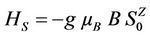
We study a single central spin atom coupled to an antiferromagnetic spin bath environment subjected to a time dependent magnetic field. Without the external magnetic field, an anti-ferromagnetic crystal has in any elementary chain two network of spin orientation; anti-parallel spin oriented in  direction and in
  direction and an anisotropy field,
 . In the presence of the external magnetic field the Hamiltonian is given for example by Equation 2.6.2 in ref. [23] The Hamiltonian of the environment used in this work is the Ising type model.
 (2.1)
(2.1)
In an anti-ferromagnetic environment contrary to the ferromagnetic environment, the coupling factor  is positive.
 (2.2)
(2.2)
 (2.3)
(2.3)
 (2.4)
(2.4)
and the magnetic moment of each atom
 (2.5)
(2.5)
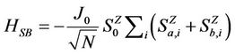
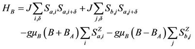
where g is the gyromagnetic factor,  is the Bohr magneton,
  the coupling constant,
  the exchange interaction. We consider only nearest neighbor interaction. We assumed that the spin structure of the environment may be divided into two interpenetrating sublattices
  and
and  with the property that all nearest neighbor of an atom of
  lie on
  and vice versa.
  and
and  represents spin operators of
  and
and  atom on sublattice a and b, each sublattice contains
  atoms.
  is the applied external magnetic field in the z-direction.
  is the anisotropy field, assumed to be positive which approximates the effect of the crystal anisotropic energy with the property of turning for positive magnetic moment,
  , to align the spins on sublattice
  in the positive z-direction and spins on sublattice
  in the negative z-direction. In ref. [24] is analyzed the crossover factor,
 ; the vector that connect(connects) atom on site
  or
or  with its nearest neighbor. To map the spin operators of the environment to bosonic operators, we use the Holstein-Primakoff transformation,
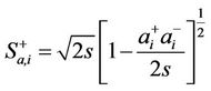 (2.6.a)
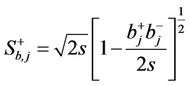 (2.6.b)
and
 (2.6.c)
 (2.6.d)
From where we have
 (2.7)
(2.7)
with  the eigen value of spin Hence Equation (2.3) defines the Heisenberg Hamiltonian plus the external magnetic field in the Ising model. It is impossible to solve it exactly but conveniently when full advantage of the translational symmetry is considered. We need creation operators which create Bloch-like non localized excitations, in order to take translational symmetry into account. We consider one atom per unit cell and,
 ’s creates localized spin deviations at a single site. We use the spin wave approximation at low temperatures and we may expect the spin deviation quantum number to be rather small. Let
  and
and  to reduce Equation (2.5) and (2.6); if we neglect the product of four operators and denote by
  the number of nearest neighbor, the Hamiltonian of the bath follows thus
 (2.8)
(2.8)
where  is the free Hamiltonian of the environment and
  the Hamiltonian describing the excited state of the environment
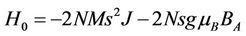 (2.9)
(2.9)
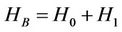
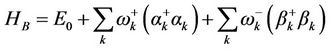
The Hamiltonian  is made (up) of two parts
 (2.10)
where the first part  is the quantified Hamiltonian of the two magnons without interaction and
  the interacting Hamiltonian of the two magnons with expressions:
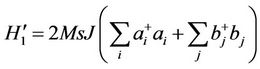 (2.11)
and
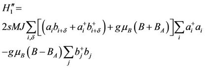 (2.12)
To find the total number of magnons, we do the Fourier transformation of the total Hamiltonian with the Bloch operators:
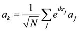 (2.13.a)
 (2.13.b)
where  is the vector of the primitive cell, k the wave vector. Let’s consider the restriction to the first Brillion zone and taking the inverse transformation of Equations (2.13.a) and (2.13.b)
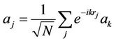 (2.14.a)
 (2.14.b)
The total number of magnons equals the total spin deviation quantum number of magnons in mode . The spin wave variable
  is substituted as
 (2.15)
where  is the occupation number operator for the number of magnons in mode k,
  is the number of particles in each sublattice and
 (2.16)
the Fourier transform coupling constant. The operators ,
,  ,
,  ,
,  are the creation and annihilation operators of sublattices
  and
and  respectively.
The Hamiltonian Equation (2.9) can then be transformed using the Bogoliubov transformation:
 (2.17.a)
 (2.17.b)
where the coefficients  and
and  are real and also the new operators obey the boson commutation rules:
 (2.18)
 (2.19)
which leads to the constraint, . The Hamiltonians respectively in Equation (2.1)-(2.3) becomes
 (2.20)
 (2.21)
 (2.22)
 is the energy of the free harmonic oscillator. The frequency of the two magnons at the symmetric position given by the site
  and the site
  of the system is:
 (2.23)
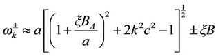
In an anti-ferromagnet Cristal, the excitation of one magnon of a wave vector k lead to a change either of + 1/N, or of –1/N for the ensemble of the two anti-parallel spins of the elementary network link. There exist then two modes,  and
and  which are degenerates if the contribution of the external magnetic field is neglected. These states, up and down correspond respectively to the eigen frequencies
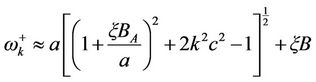 (2.24.a)
and
 (2.24.b)
From the given expressions Equations (2.24.a) and (2.24.b), we see that the magnetic state of spin “up” or “down” depends at the same time on the excitation of the modes  and
and  and to the population
  and
and  or of
or of  and
and . Using the kinetic energy expression of the system, the effective mass
  of magnon is found,
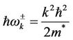 (2.25)
From where we have
 (2.26)
Equation (2.26) gives the effective mass of a quasiparticle moving in the crystal with frequencies  in mode
  where a, b, c,
  are the constants of system. The result of Equation (2.24.a) is not a good approximation to the situation of the spin wave [25]: We don’t take into account the processes which give in return their half-life. It has been calculated by some authors [26,27]. The critical magnetic field Bc (the corresponding external field that corresponds to field with the energy equals to the energy of the environment) is evaluated; that is when the mode
  and at the finite oscillating time,
 , and taking
 :
:
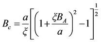 (2.27)
Equation (2.27) is the critical magnetic field obtained as for the constant external magnetic field in [28]. In analogy to the dressed atom picture [29], the eigen frequencies  can be associated with dressed states, that is, the oscillator frequencies of state
  and
and  (that are the states respectively with oscillator frequencies
 ,
, ), in the presence of mutual coupling.
In Figures 1-3 are plotted the frequencies of the two oscillators. In Figure 1 the two curves intersect at  and later diverge. The dynamics of the eigen modes frequencies as function of time shows oscillations depicting the character variability of the external magnetic field Figure 2, it appears that the two curves intersect at
The dash curve corresponds to the frequency  and the solid curve to the frequency
 .
.
There is a characteristic anti-crossing with a frequency splitting of
 (2.28)
with . As
. As , the splitting increases with the external field. Anti-crossing is a characteristic fingerprint of strong coupling.
The eigen modes of the oscillators with frequencies  translate the system to that of a two level system
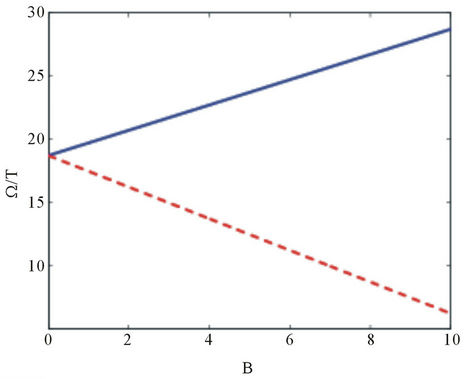
Figure 1. Plot of the frequency versus the magnetic field with the constants ,
,  ,
,  , M = 6. The dash curve corresponds to the frequency
  and the solid curve to the frequency
 .
.

Figure 2. Plot of the frequency versus time in the two states Zeeman effect.
coupled by a constant magnetic field as analogous to the case in [30] where the coupling is via a spring constant, whereby in the light of Landau-Zener scenario, the frequency difference of the oscillator changes linearly in time, the probability for level crossing (diabatic transition) at infinite large time is
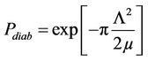 (2.29)
where  is the transition speed and is given by the dispersion relation
 , where
  is the wave vector.
Equation (2.29) is the probability that the anti-ferromagnetic bath mode remains in the initially prepared state . The characteristic Gaussian shape of this transition is shown in Figure 3(a) a signature that the antiferromagnetic spin bath described by the two frequency modes interact via the magnetic field with the subsequent collapse of population with frequency mode
  (red solid curve) and raising of population with frequency mode
  (green solid curve). This implies the magnetic field provides means by which the anti-ferromagnetic spin bath could be tailored.
In Figure 3(b) supposing , the plot shows the range of values of the phase angle
  that the survival transition amplitude is maximum as it exhibits a resonant peak. There is shrinkage in the width of this resonant peak for large value of the magnetic field
 (a)
(a)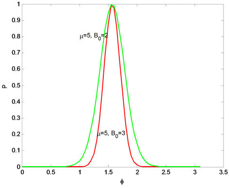 (b)
(b)
Figure 3. (a) Diabatic transition probability versus constant magnetic field , with
 ; (b) Diabatic transition probability versus phase angle for arbitrary
 , with
 .
.
amplitude implying the initially prepared state of the environmental frequency mode could be tailored with precision if a certain value of the magnetic field amplitude and phase angle is used. Figure 4 is the plot of the frequency versus the wave vector for some system parameters. The dotted curve represents the behavior of the frequency,  and the solid curve that of the frequency,
  as the wave vector is varied. These curves show a basin-like behavior. It proceeds two extreme values (or minima) corresponding to the high cut-off frequency and the low cut-off frequency. Thus, any wave which is propagated with a frequency not included in this domain vanishes. Note that we have ignored damping of the magnons in the analysis of the coupled oscillators. When the external magnetic field exceeds Bc, we have
 . This indicates that, this branch of magnon is no longer stable due to the externally applied magnetic field.
As a result, the anti-ferromagnetic polarization flips perpendicular to the field, i.e., the magnetic field induces spin flop transition. The spin-flop transition demonstrates a significant change of the spin configuration in the anti-ferromagnetic environment. This phenomenon has been observed and investigated for many different materials [31-33]. The spin wave theory is known to describe well the low-excitation and low-temperature properties of anti-ferromagnetic materials.
Despite this low-excitation approximation, the spin wave theory also describes well the physics for  and the value of the critical magnetic field of the spin-flop transition in anti-ferromagnetic materials [28]. We will thus use the spin wave theory to discuss the decoherence time of the central spin under the influence of the anti-ferromagnetic environment when the external magnetic field is tuned to approach
  from below (i.e.
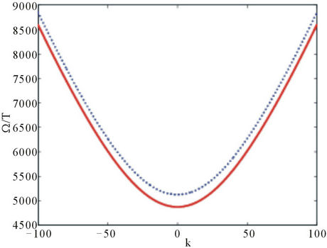
Figure 4. Frequency versus the wave vector, with different constants: ,
,  ,
,  , M = 6, B = 2, in the two state of the Zeeman effect.
 for
for ). It will be shown that an analytic expression for the decoherence time can be evaluated.
3. Decoherence Time
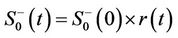
In this section, using the time evolution of the off-diagonal elements of the reduced density matrix for the central spin, we calculate the decoherence time. We assumed factorized initial state of the density matrix of the total systems, i.e.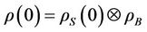 . The initial state of the central spin is described by
 . The density matrix of the environment is assumed to be in thermal equilibrium, that is
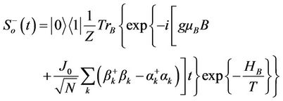
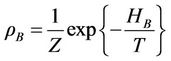 , where Z is the partition function. We are interested in the dynamics of the off-diagonal elements of the reduced density matrix as they carry information on the phase coherence of the system. This is equivalent to calculating the time evolution of the spin-flip operator,
  , where
  and
and  are respectively the lower and upper eigen states of
 . By tracing out the environmental degrees of freedom, the time evolution of
  can be written as:
 (3.30)
 (3.30)
the decoherence factor  can be found using the time evolution
 (3.31)
From Equation (2.3) the decoherence factor yields
 (3.32)
where
 (3.33.a)
 (3.34.b)
The decoherence factor of the system in the volume  of environment is found at low temperature; that is for
 , where
  is the temperature,
 (3.35)
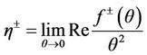
Then in the thermodynamic limit, i.e. ,
,  it is obvious that
  as
as . To find the relation between
  and
and  in the thermodynamic limit, we calculate:
 (3.36)
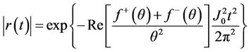
The absolute value of the decoherence factor in the thermodynamic limit can be expressed:
 (3.37)
where
 (3.38)
We obtained these results analytically for the case of a variable magnetic field. It indicates that the decoherence factor displays a Gaussian decay with time (see Equation (3.37)). The factor  in the exponent is different from the Markovian approximation which usually shows a linear decay in time in the exponent thus portraying nonMarkovianity a signature of strong coupling between system and environment.
In Figure 5 we see that the decoherence time decreases monotonically to zero with the external magnetic field. The opposite is observed in Figure 6 where the
Figure 5. Decoherence time versus the external magnetic field, with different constants: ,
,  , BA = 0.014, M = 6,
 .
.
Figure 6. Plot of the decoherence time versus the anisotropy field, with the chosen constants ,
,  , B = 0.1, M = 6,
 .
.
decoherence time increases exponentially with the anisotropy field. This behavior shows the fact that the anisotropy gives rise to stronger polarization of the environmental spin and reduces the effect of the external field on the decoherence of the central spin.
As discussed in[13] the field-dependent decoherence behavior may be inferred from the effective Hamiltonian, Equations (2.24)-(2.26). From the interaction Hamiltonian, Equation (2.25), we see that the larger the difference in the magnon excitation number between the magnon  and magnon
 , the stronger the effect of the environment on the central spin. At a given temperature, the average thermal excitation number may be the same for the two magnons, but the fluctuation in the excitations for each individual magnon may not be the same at the same time. If the external magnetic field is increased, the magnon frequency
  decreases but
  increases. Consequently, the magnon mode
  is easier to be excited than the magnon mode
  at a given anisotropy field, temperature and time. This results in a larger magnon excitation number difference and fluctuation, and thus a stronger decoherence effect.
An alternative way to understand the field-dependent decoherence time may be in terms of quantum correlations. There is a kind of trade-off between the external magnetic field and the anisotropy field. The anisotropy field renders the anti-ferromagnetic environment stable. On the other hand, the external magnetic field tends to reduce the anti-ferromagnetic order of the environment. Therefore the stronger the external magnetic field is, the smaller the anti-ferromagnetic order. On the contrary, the larger the anisotropy field is, the stronger the correlation of the anti-ferromagnetic environment. If the constituents (spins) of the environment maintain appreciable correlations or entanglement between themselves, then there is a restriction on the entanglement between the central spin and the environment [34,35]. As a consequence, this sets a restriction on the amount that the central spin may decohered [32,33,36]. Thus as far as the decoherence of the central spin is concerned, the anisotropy field has a similar effect on the exchange interaction strength between the constituents (spins) of the anti-ferromagnetic environment. Strong intra-environmental interaction results in a strong anti-ferromagnetic correlation, thus an effective decoupling of the central spin from the environment and a suppression of decoherence [32,33]. Therefore the decoherence time increases with the increase of the anisotropy field but decreases with the increase of the strength of the external magnetic field.
In the subsequent section we find the transition probability of state in the system, considering that the density matrix of the environment is in thermal equilibrium.
4. Probability Density of State
At thermodynamic equilibrium, the density state of the system is expressed as
 (4.39)
H is the total Hamiltonian and T the Boltzmann temperature. Let’s evaluate the partition function of the system, at the thermodynamic equilibrium
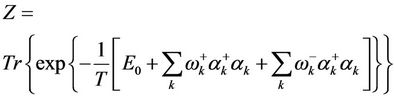 (4.40)
Here, g is the gyromagnetic factor, E0 the energy of the free harmonic oscillator.
If we let ,
,  the number of magnon for the different creation operator
  and
and  respectively
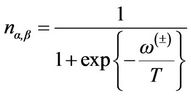 (4.41)
Then we have the mean value of the probability density of state.
 (4.42)
where
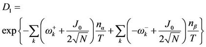 (4.43)
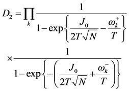 (4.44)
The solid curve represents the vibration mode with frequency  and the dot curve the mode with frequency
 . Here,
  is the gap between the two vibrational modes where looking at Equation (2.28), it results that
  and may be interpreted as the energy necessary for spin transition from low spin energy state to high energy spin state.
Figures 7-9 show plots of the probability density of state as a function of temperature. The plots demonstrate a resonance peak within some temperature range. This provides us with additional information on the range of values of the temperature, anisotropy field, magnetic field and other system parameters for which the central spin system is sensitive to and possibly undergoes transition. Transforming temperature into frequency via the Matsubara relation, we could talk of triple resonance comprising of the driving field frequency, anisotropy field frequency and the environmental eigen modes frequency. The resonance peak in the plot of the probability density of state for the two vibrational modes corresponds to minimum decoherence effect of the environment and the driving field on the central spin. In Figure 7, it is seen that two different peaks having the same magnitude arises for the two eigen modes frequencies ,
,  at different temperatures. We see that the two different modes enhance the probability density of state with each doing so at different temperature ranges. In the same figure
  is the gap between the two vibrational modes where by looking at Equation
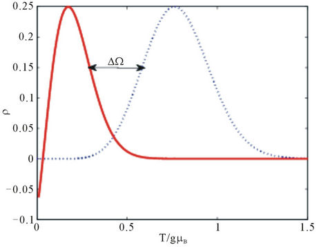
Figure 7. Plot of the probability density versus the temperature.
(2.29), it results that  and may be interpreted as the energy necessary for spin to make transition from its low energy state (with frequency mode
 ) to its high energy state (with frequency mode
 ) and vice versa. In Figure 8 it is seen that the variable external magnetic field reduces the probability density of state as compared to the constant magnetic field. The character variability of the external magnetic field with its frequency is used to control the dynamic of the hold system. This is because the variable field induces oscillations amongst the magnon modes with alternate collapse and revival of the modes. In Figure 9, the anisotropy field plays the inverse rule as compared to the external magnetic field.
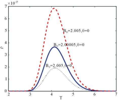
Figure 8. Probability density of state for a central spin in an antiferromagnetic spin system versus temperature for different value of the external field. With BA = 1.5.

Figure 9. Plot of probability density of state for a central spin in an antiferromagnetic spin system versus temperature for different anisotropic magnetic field. With B0 = 2.
That is, the stronger the anisotropy field, the stronger the decoherence of the central spin system.
The solid and dash curves are the plot considering the external magnetic field constant whereas the dotted curve is the plot of the probability density of state subjected to a variable magnetic field.
We observed from Figure 8 that increasing the anisotropic magnetic field intensity leads to an increase in the amplitude of the probability density. This shows that the anisotropy field provides to the central spin a decoherence free environment. This behavior is not surprising as the decoherence time increases with increase in anisotropy (see Figure 6).
5. Conclusion and Perspective
We have studied the decoherence of a central spin coupled to an anti-ferromagnetic environment in the presence of a variable external magnetic field. The results, obtained using the spin wave approximation in the thermodynamic limit, show that the decoherence factor displays a Gaussian decay with time. It is shown that the probability density of state occurs at some critical values of magnetic field and temperatures. The probability density as a function of temperature is characterized by a resonant peak corresponding to some critical parameters of the system which here are the critical external magnetic field, anisotropy field and temperatures. The probability of the central spin to remain in the initially prepared state is maximum at these values and spin-flop transition is suppressed. Out of these parameter range spin-flop transition occurs, consistent with the QPT as studied in [37-39]. It is equally seen that strong anisotropy field enhances the probability density and reduces decoherence of the anti-ferromagnetic environment of the central spin. Therefore, in order to reduce the loss of coherence of the central spin, we could decrease the environmental temperature, choose variable magnetic field with high amplitude (which) could lead to dark state of the environment, and choose the anti-ferromagnetic surrounding or underlying anti-ferromagnetic materials with a strong crystal anisotropy field. The frequency eigen mode dependence on the phase angle as shown in (Figure 3(b)) suggest to us that the transition amplitude strongly depend on the phase angle and shall be one of the aspects for our future investigation.
REFERENCES
- D. Guilini, E. Joos, C. Kiefer, J. Kupsch, I. O. Stamatescu and H. D. Zeh, “World in Quantum Theory,” SpringerVerlag, Berlin Heidelberg, 1996.
- R. R. Chance, A. Prock and R. Silbey, “Molecular Fluorescence and Energy Transfer near Metal Interfaces,” Advances in Chemical Physics, Vol. 37, 1978, pp. 1-65. doi:10.1002/9780470142561.ch1
- E. M. Purcell, “Spontaneous Emission Probabilities at Radio Frequencies,” Physical Review, Vol. 69, 1946, p. 681.
- Th. Förster, “Zwischenmolekulare Energiewanderung und. Fluoreszenz,” Annalen der Physik, Vol. 437, No. 1-2, 1948, pp. 55-75. doi:10.1002/andp.19484370105
- G. W. Ford, J. T. Lewis and R. F. O’Connell, “Quantum Measurement and Decoherence,” Physical Review A, Vol. 64, No. 3, 2001, Article ID: 032101. doi:10.1103/PhysRevA.64.032101
- A. Venugopalan, “Pointer States via Decoherence in a Quantum Measurement,” Physical Review A, Vol. 61, No. 1, 1999, pp. 012102-012109. doi:10.1103/PhysRevA.61.012102
- G. Dominique, D. V. Jan and A. Vinay, “Comment on Quantum Measurement and Decoherence,” Physical Review A, Vol. 70, No. 2, 2004, pp. 1-4. doi:10.1103/PhysRevA.70.026101
- V. Ambegaokar, “Negotiating the Tricky Border between Quantum and Classical,” Physics Today, Vol. 46, No. 4, 1993, p. 82.
- R. ADAMI and C. Negulescu, “A Numerical Study of Quantum Decoherence,” Communications in Computational Physics, Vol. 12, 2012, pp. 85-108. doi:10.4208/cicp.011010.010611a
- R. Adami and L. Erdȍs, “Rate of Decoherence for an Electron Weakly Coupled to a Phonon Gas,” Journal of Statistical Physics, Vol. 132, 2008, pp. 301-328. doi:10.1007/s10955-008-9561-8
- A. Bertoni, “Simulation of Electron Decoherence Induced by Carrier-Carrier Scattering,” Journal of Computational Electronics, Vol. 2, 2003, pp. 291-295. doi:10.1023/B:JCEL.0000011440.86454.13
- L. Novotny and B. Hecht, “Principles of Nano-Optics,” Cambridge University Press, Cambridge, 2006. doi:10.1017/CBO9780511813535
- Y. Xiao-Zhong, G. Hsi-Sheng and Z. Ka-Di, “Influence of an External Magnetic Field on the Decoherence of a Central Spin Coupled to an Antiferromagnetic Environment,” New Journal of Physics, Vol. 9, 2007, p. 219. doi:10.1088/1367-2630/9/7/219
- C. L. Garrido Alzar, M. A. G. Martinez and P. Nussenzveig, “Classical Analog of Electromagnetically Induced Transparency,” American Journal of Physics, Vol. 70, No. 1, 2000, p. 37. doi:10.1119/1.1412644
- W. Frank and P. von Brentano, “Classical Analogy to Quantum Mechanical Level Repulsion,” American Journal of Physics, Vol. 62, No. 8, 1994, pp. 706-709. doi:10.1119/1.17500
- H. J. Maris and Q. Xiong, “Adiabatic and Nondiabatic Processes in Classical and Quantum Mechanics,” American Journal of Physics, Vol. 56, No. 12, 1988, pp. 1114- 1117. doi:10.1119/1.15734
- B. W. Shore, M. V. Gromovyy, L. P. Yatsenko and V. I. Romanenko, “Simple Mechanical Analogs of Rapid Adiabatic Passage in Atomic Physics,” American Journal of Physics, Vol. 77, No. 12, 2009, pp. 1183-1194.
- C. H. Bennett, G. Brassard, C. Crépeau, R. Jozsa, A. Peres and W. K. Wootters, “Teleporting an Unknown Quantum State via Dual Classical and Einstein-PodolskyRosen Channels,” Physical Review Letters, Vol. 70, 1993, pp. 1895-1899. doi:10.1103/PhysRevLett.70.1895
- D. Bouwmeester, J. W. Pan, K. Mattle, M. Eibl, H. Weinfurter and A. Zeilinger, “Experimental Quantum Teleportation,” Nature, Vol. 390, 1997, pp. 575-579. doi:10.1038/37539
- C. H. Bennett, G. Brassard and A. K. Ekert, “Quantum Cryptography,” Scientific American, Vol. 267, No. 4, 1992, pp. 50-57. doi:10.1038/scientificamerican1092-50
- C. H. Bennett and S. J. Wiesner, “Communication via Oneand Two-Particle Operators on Rosen states,” Physical Review Letters, Vol. 69, 1992, pp. 2881-2884. doi:10.1103/PhysRevLett.69.2881
- M. Murao, D. Jonathan, M. B. Plenio and V. Vedral, “Quantum Telecloning and Multiparticle Entanglement,” Physical Review A, Vol. 59, No. 1, 1999, pp. 156-161. doi:10.1103/PhysRevA.59.156
- H. Le Gall, “Dynamique de Spin et Interactions Spin-PhoTon,” Revue de Physique Appliquée, Vol. 9, No. 5, 1974, pp. 793-818. doi:10.1051/rphysap:0197400905079300
- G. Jona-Lasinio, C. Presilla and C. Toninelli, “A Mean Field Model and Comparison with Experiments,” Physical Review Letters, Vol. 88, 2002, Article ID: 123001. doi:10.1103/PhysRevLett.88.123001
- R. Silbey and R. A. Harris, “Variational Calculation of the Dynamics of a Two Level System Interacting with a Bath,” Journal of Chemical Physics, Vol. 80, No. 6, 1984, p. 2615. doi:10.1063/1.447055
- P. G. de Gennes “Nuclear Magnetic Resonance Modes in Magnetic Material. I. Theory,” Physical Review, Vol. 129, No. 3, 1963, pp. 1105-1115. doi:10.1103/PhysRev.129.1105
- U. Upadhyaya and K. Sinha, “Phonon-Magnon Interaction in Magnetic Crystals. II. Antiferromagnetic Systems,” Physical Review, Vol. 130, No. 3, 1963, pp. 939- 944. doi:10.1103/PhysRev.130.939
- K. Yosida, “Theory of Magnetism,” Springer Series in Solid-State Sciences, Vol. 122, 2010, 320 p.
- C. Cohen-Tannoudji, J. Dupont-Roc and G. Grynberg, “AtomPhoton Interactions,” Wiley-VCH Verlag, Weinheim, 2004.
- L. Novotny and Strong Coupling, “Energy Splitting, and Level Crossings: A Classical Perspective,” University of Rochester, Rochester, 2010.
- S. Yunoki, “Numerical Study of the Spin-Flop Transition in Anisotropic Spin-1/2 Antiferromagnets,” Physical Review B, Vol. 65, No. 9, 2002, Article ID: 092402. doi:10.1103/PhysRevB.65.092402
- A. L. Dantas, S. R. Vieira, N. S. Almeida and A. S. Carrico, “Soft Mode of Antiferromagnetic Multilayers near the Surface Spin-Flop Transition,” Physical Review B, Vol. 71, No. 1, 2005, Article ID: 014409. doi:10.1103/PhysRevB.71.014409
- D. Joonghoe, C. W. Leung, Z. H. Barber and M. G. Blamire, “Competing Functionality in Multiferroic YMnO3,” Physical Review B, Vol. 71, No. 18, 2005, Article ID: 180402.
- Y. Xiao-Zhong, G. Hsi-Sheng and Z. Ka-Di, “Dynamics of a Driven Spin Coupled to an Antiferromagnetic Spin Bath,” New Journal of Physics, Vol. 13, 2011, Article ID: 023018. doi:10.1088/1367-2630/13/2/023018
- H. Hwang and P. J. Rossky, “An Analysis of Electronic Dephasing in the Spin-Boson Mode,” Journal of Chemical Physics, Vol. 120, No. 24, 2004, Article ID: 11380. doi:10.1063/1.1742979
- S. Paganelli, F. De Pasquale and S. M. Giampaolo, “Decoherence Slowing down in a Symmetry-Broken Environment,” Physical Review A, Vol. 66, No. 5, 2002, Article ID: 052317.
- H. T. Quan, Z. Song, X. F. Liu, P. Zanardi and C. P. Sun, “Decay of Loschmidt Echo Enhanced by Quantum Criticality,” Physical Review Letters, Vol. 96, 2006, Article ID: 140604. doi:10.1103/PhysRevLett.96.140604
- F. M. Cucchietti, S. Fernandez-Vidal and J. P. Paz, “Universal decoherence induced by an environmental quantum phase transition,” Physical Review A, Vol. 75, No. 3, 2007, Article ID: 032337. doi:10.1103/PhysRevA.75.032337
- P. Zanardi, H. T. Quan, X. G. Wang and C. P. Sun, “MixedState Fidelity and Quantum Criticality at Finite Temperature,” Physical Review A, Vol. 75, No. 2007, pp. 1-7.
NOTES
*Corresponding author.