ABSTRACT

To evaluate the pollutant dispersion in background turbulent flows, most researches focus on statistical variation of concentrations or its fluctuations. However, those time-averaged quantities may be insufficient for risk assessment, because there emerge many high-intensity pollutant areas in the instantaneous concentration field. In this study, we tried to estimate the frequency of appearance of the high concentration areas in a turbulent flow based on the Probability Density Function (PDF) of concentration. The high concentration area was recognized by two conditions based on the concentration and the concentration gradient values. We considered that the estimation equation for the frequency of appearance of the recognized areas consisted of two terms based on each condition. In order to represent the two terms with physical quantities of velocity and concentration fields, simultaneous PIV (Particle Image Velocimetry) and PLIF (Planar Laser-Induced Fluorescence) measurement and PLIF time-serial measurement were performed in a quasi-homogeneous turbulent flow. According to the experimental results, one of the terms, related to the condition of the concentration, was found to be represented by the concentration PDF, while the other term, by the streamwise mean velocity and the integral length scale of the turbulent flow. Based on the results, we developed an estimation equation including the concentration PDF and the flow features of mean velocity and integral scale of turbulence. In the area where the concentration PDF was a Gaussian one, the difference between the frequencies of appearance estimated by the equation and calculated from the experimental data was within 25%, which showed good accuracy of our proposed estimation equation. Therefore, our proposed equation is feasible for estimating the frequency of appearance of high concentration areas in a limited area in turbulent mass diffusion.

Keywords:

High Concentration Spikes, Quasi-Homogeneous Turbulence, Turbulent Mass Diffusion, Concentration PDF Transport Equation, PIV and PLIF Simultaneous Measurement

1. Introduction

Turbulent diffusion research has been taken seriously for many years, with one reason that turbulent flow plays an efficient role in most of the pollutant spread in natural environment. When pollutant leakage happens, identification of the leakage source, prediction of the possible damage regions and evacuation of people in these regions must race against time. To save rescue time and reduce damage, a quick and accurate method of predicting pollutant diffusion in the turbulent flow is needed. In the case of the Fukushima Daiichi Nuclear Power Plant disaster in 2011, the “System for Prediction of Environmental Emergency Dose Information” was applied in order to predict the dispersion of radioactive material emitted from the nuclear power plant [1] [2] [3] . The development of a prediction method for turbulent mass diffusion has been studied by many researchers [4] [5] [6] . Basically, the transport equation for the time-average concentration field of the material is solved numerically to predict the diffusion of the pollutant material. However, for the diffusion phenomena in a turbulent flow, the diffusion prediction with the time-average concentration distribution is not enough to quantify the damage of the pollutant diffusion accurately. The reason for this is that the concentration of the pollutant material fluctuates in both space and time, and areas with a high concentration and a high concentration gradient compared with the surroundings (hereafter the areas are high concentration spikes) are formed by the organized structure of the turbulent flow when the pollutant material spreads. These high concentration spikes have higher instantaneous concentration than the time-average concentration, and this can lead to heavy damage. Accordingly, a quick and accurate method of estimating the dispersion of the high concentration spikes in a turbulent flow is of great importance.

The high concentration spikes have been attracting the interest of a number of researchers in past studies. Page et al. [7] devised a method of extracting high concentration spikes from time-serial data on the material concentration using the concentration threshold. Webster et al. [8] reported that both mean concentration in the high concentration spikes and the frequency of appearance of the spikes decrease with the downstream distance from the source. This knowledge was also used to estimate the diffusion source of the material diffusing in a turbulent flow. In our previous studies [9] [10] , a unique technique was used to extract the high concentration spikes from the plume in a quasi-homogeneous turbulent flow and the diffusion process of the high concentration spikes was investigated. From the scalar statistics of the high concentration spikes, including the mean concentration, the length scale and the diffusion coefficient, it was clear that the diffusion process of the spikes was greatly affected by the meandering diffusion in the turbulent flow, which differed from regular mass diffusion. Moreover, the high concentration spikes were found to be repeatedly formed in a turbulent flow. According to [11] [12] , the formation of the spikes happened at a saddle point of the velocity field caused by the large scale structure of the turbulent eddies. Considering that the formation of the high concentration spikes in a turbulent flow occurs and the spike is extracted based on the concentration value as well as the concentration gradient value, it can be suspected that the behavior of the spikes follows a totally different diffusion law from a regular mass diffusion in a turbulent flow. Although the diffusion and formation mechanisms of the spikes are increasingly obvious, there is no simple method of estimating the turbulent dispersion of the spikes, and therefore the development of such as method is very important.

In this study, we tried to develop the equation to estimate the dispersion of the high concentration spikes by using physical parameters and evaluated the estimation equation. We employed the frequency of appearance of the spikes as a parameter to describe the dispersion of the spikes. The frequency of appearance denoted the number of spikes observed at a fixed point per unit time when the diffusing material concentration was continuously measured at the point. In a turbulent flow, estimating the frequency of appearance of the spikes with limited available information, such local mean velocity and local mean concentration, can be useful to estimate the damage caused by the pollutant material diffusion. With the purpose of representing the estimation equation for the frequency of appearance as physical parameters of the turbulent mass diffusion, we experimentally demonstrated the concentration field of a passive scalar diffusing from a point source in a turbulent water flow. As a simple case, we employed a channel flow which had quasi-homogeneous turbulence at the center of the channel. Although such an ideal turbulent flow is rare in the atmospheric boundary layer as well as in other practical situations, we investigated the capability of our simple estimation trial focusing on the neutrally-stratified core region of a turbulent channel flow.

The next section presents the concept of the estimation equation we proposed in this paper. Section 3 describes our experimental setup to demonstrate the passive-scalar turbulent diffusion. Based on the experimental data, physical parameters are confirmed to be useful to represent the estimation equation in Section 4.1, Section 4.2, and Section 4.3. The results of the diffusion estimation of the spikes and its proposition are presented in Section 4.4.

2. Concept and Development of Estimation Equation

In this section, we describe the concept and the configuration procedure of our proposed equation for estimating the frequency of appearance of high concentration spikes. To observe the high concentration spike in a turbulent mass diffusion, we performed experiments on the turbulent dispersion of a matter (dye) emitted continuously from a fixed source in a three-dimensional turbulent flow, although we considered it as a two-dimensional flow. We mainly focused on the horizontal diffusion in the central plane of the channel rather than on the wall-normal (y) diffusion.

The position and the area of the high concentration spikes in the diffusing dye were recognized with the conditional sampling technique proposed in [9] [10] , which has two conditions. Figure 1 shows an example of the experimental and the analytical results. Here, the superscript of * indicates normalization by the channel half width, i.e., z^* = z/δ. Figure 1(a) is a typical snapshot of the diffusing dye, obtained by PLIF measurement.

In Figure 1(a), greater brightness means higher fluorescent intensity, which is proportional to the local dye concentration, showing dye plumes with low and high concentration areas. Figure 1(b) shows the corresponding binarized image marking the position of the high concentration spikes, obtained by the conditional sampling technique. The white areas in Figure 1(b) stand for high concentration spikes, while the

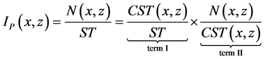
black areas indicate zero or low concentration areas. The frequency of appearance of the high concentration spikes I_P corresponds to the number of the white areas observed at any fixed point during the period the dye concentration was sampled. An example of experimental time-serial concentration data is shown in Figure 2. In Figure 2, the horizontal axis denotes the sample observation time, while the vertical axis denotes observed instantaneous concentration. The red line in the graph shows the sum value of the time-average concentration and the concentration fluctuation intensity.

The value N is the number of spikes for a fixed point in the x-z plane during a sampling time, and is defined as the total number of points with local maximum concentration which is larger than the red line from Figure 2. In addition, ST denotes the sampling time, while CST denotes the conditional sampling time, which equals the total time of the experimental durations when the instantaneous concentration is over the red line. Assuming that the concentration field was steady, the frequency of appearance of the spikes I_P is independent of time, and is defined by

(1)

In order to estimate the frequency of appearance without any experimental observed data on the concentration, which is our purpose, a new expression is necessary for the definition of Equation (1) with limited available information such as concentration and flow features. We employed two conditions for the concentration and the concentration gradient values in order to identify the existence of the high concentration spikes in the diffusing dye image. One condition for the concentration value recognized the area having a larger instantaneous concentration than the threshold corresponding to

the sum of the time-average concentration and the concentration fluctuation intensity in the time-serial observation data. Another condition for the concentration gradient value recognized the interval between the point of the maximum concentration gradient and the point of the minimum concentration gradient. We consider that Equation (1) can be decomposed into two constituent terms based on the two conditions because the two conditions should be independent of each other. Therefore, our proposed estimation equation of I_P can be rewritten by

(2)

Accordingly, in Equation (2), the first term of CST/ST on the right side shows the probability that the observed concentration will meet the condition for the concentration value, and the second term of N/CST on the right side shows the ratio of the number of the spikes to CST. Hereafter, the first and second terms are named “term I” and “term II” respectively. Based on the new expression with the two terms, the diffusion estimation of the high concentration spikes without any observation needs a method of physically representing the two terms with available experimental data on the velocity and concentration fields.

To represent the term I in Equation (2) with a physical parameter, we adopt the PDF of concentration, f_ϕ. By analogy, term I can be represented with the integration of the concentration PDF,

(3)

Pope [13] proposed the transport equation for the concentration PDF, shown in Equation (4), with the transport equation for the concentration in Equation (5) and Dirac’s delta function. The solution of the transport equation provides the spatial distribution of the concentration PDF.

(4)

(5)

where denotes an instantaneous velocity [m/s], which can be separated into a time-average velocity and a velocity fluctuation, while c denotes the instantaneous concentration. In addition, D is a molecular diffusion coefficient [m²/s]. The terms and respectively denote the conditional velocity fluctuation and the conditional dissipation rate based on the condition of the instantaneous concentration. The modeling of the two conditional values is necessary to solve the transport equation of the concentration PDF, and has been studied in many researches [14] [15] [16] . We calculated the conditional velocity fluctuation and the conditional dissipation rate through an experiment of simultaneously measuring the velocity and the concentration distributions in a two-dimensional plane, and discussing the limit of modeling of the two conditional values in this study. Moreover, for term II, a comparison between term II calculated from the time-serial measurement of the concentration and term II estimated with the physical parameters of the flow features as well as the concentration fields was performed. A simple method of representing term II physically was developed.

3. Experimental Procedure

Figure 3 shows our main experimental apparatus, which was a closed-circuit water channel. The water flow under constant temperature was driven by an inverter-con- trolled centrifugal pump with a constant volume. A rectifier was installed at the entrance to ensure a steady flow by damping the large vortices. The channel part including the measurement section was made of transparent acrylic resin for precise visualization and had a height of 20 mm (2δ), and a width of 250 mm (aspect ratio 12.5). A fully developed two-dimensional turbulent channel flow was established in the measurement section, which was located 2000 - 3000 mm downstream from the channel inlet. The flow rate Q was measured by a flow-meter to monitor the Reynolds number. The bulk Reynolds number was fixed at, where and ν denote the bulk velocity and the kinematic viscosity of water, respectively. In this study, we focus on statistically modeled quasi-homogeneous turbulence as a simple case for estimating the frequency of appearance of high concentration spikes. Accordingly, the uniformity of the time-average velocity and the turbulent intensity in the turbulent flow are important. Figure 4 shows the spanwise distributions of time-average streamwise velocity and turbulent intensity at the channel center obtained by PIV measurement. We were able to confirm that the velocity field in the measurement area was fully developed and there was no significant gradient in the spanwise direction. This

means that the flow field we focused on in this study had quasi-homogeneous turbulence in the two-dimensional plane of the streamwise and spanwise directions.

In order to measure the spatial velocity field and concentration field at the same time and at the same position and to calculate the conditional velocity fluctuation and conditional dissipation rate, we employed simultaneous PIV and PLIF measurement. This simultaneous measurement was extensively used to investigate the turbulent mixing processes [17] [18] [19] . However, in the simultaneous measurement, the time step of the photographing images is too large to precisely calculate the number of high concentration spikes in a time series data and term II. Therefore, PLIF time-serial measurement was carried out to observe the temporal fluctuation of the concentration field with the short time step. Figure 5 and Figure 6 respectively show the measurement sections of the simultaneous PIV and PLIF measurement and the PLIF time-serial measurement. For the latter, Rhodamine-WT solution with a high Schmidt number of approximately 3000 in water was injected as a dye into the water flow from a nozzle which was aimed downstream and positioned at the center of the channel.

The nozzle had an internal diameter of 1 mm and outside diameter of 2 mm. Both coordinate systems define x as the streamwise direction, z as the spanwise direction, y as the vertical direction and the nozzle tip as the origin point. The injection speed of the dye solution was controlled by a micro-syringe pump and kept the same as the velocity of the local flow. We assumed that the volume of released dye solution was so small that any effects on the turbulence might be neglected. On illumination by laser light with a wavelength of 532 nm, the dye on the illuminated plane emitted fluorescent light with a wavelength of 580 nm, the strength of which was captured by a high speed camera (Photoron FASTCAM-APX RS250K) as a PLIF image after being filtered by a color filter (HOYA colored optical glass O54). The laser illuminated plane was set at half the height of the channel. A laser emission device (CW:YAG laser) was installed at the side of the channel while a high speed camera to capture the light for measurement of concentration was installed below the channel. Therefore, this measurement provided the time-

series data of the two-dimensional images of dye diffusion in the streamwise and spanwise directions. The concentration of the dye was calculated assuming that the fluorescent intensity was proportional to the local dye concentration. The photographic frame rates were 1000 and 3000 fps, and the number of consecutive images for statistics was 1000. For simultaneous PIV and PLIF measurement, tracer particles with average diameter of 20 μm were seeded into the flow. With the same injection of the dye solution and laser illumination as in the PLIF case, scattering light from the tracer particle and fluorescent light from the dye were captured by the CCD camera (Flow Sense 4M), after being separated by a beam splitter. We used an Nd:YAG laser as a laser emission device, which emitted laser light with the same wavelength of the CW:YAG laser. In this experiment, the photographic frame rate was 4 fps and 1000 consecutive images were captured simultaneously. The simultaneous PIV and PLIF measurements were taken at a sequence of streamwise distances x = 5δ, 10δ, 20δ, 35δ, 40δ, 45δ, and 60δ, while the PLIF time-serial measurement were taken at a sequence of streamwise distances x = 5δ, 10δ, 15δ, 25δ, 35δ, 40δ, 45δ, 50δ, and 60δ, in order to acquire the spatial concentration and velocity distributions at various downstream distances from the nozzle. The photographed area was approximately 4.75δ × 4.75δ in size with a spatial resolution of 0.04δ in the simultaneous measurement, while the area was approximately 9.5δ × 9.5δ with a spatial resolution of 0.01δ in the time-serial measurement, which was enough to resolve fine-scale eddies in the turbulent flow. The mixing-length scale in the outer layer of wall turbulence was roughly estimated as 0.09δ [20] . Compared to the mixing-length scale, the present spatial resolution is fine enough. As for the size of measurement area, the present condition covers large-scale eddies in the turbulent flow. As a reference, note that the streamwise integral length scale obtained by integration of the streamwise two-point correlation coefficient of velocity field was about 0.7δ.

4. Results and Discussion

4.1. Conditional Velocity Fluctuation

In this section, the conditional velocity fluctuation in the transport equation of the concentration PDF is calculated from the experimental data with the simultaneous PIV and PLIF measurement, and the limits of modeling the conditional velocity fluctuation are discussed. The conditional velocity fluctuation means the ensemble average of velocity fluctuations conditional on the associated value ψ being at a chosen value c. In this paper, normalized conditional velocity fluctuation and normalized concentration Ф are defined by,

(6)

where i is an indicator of velocity direction, i.e., and. According to Pope [13] , when the joint PDF of the velocity and the concentration was normal, the normalized conditional velocity fluctuation had a linear relationship with normalized concentration Ф, which was given by,

(7)

The explanation was that when at a certain position a fluid parcel was found with a concentration which deviated strongly from the local mean concentration, the absolute value of the velocity of this parcel differed strongly from the mean. Moreover, Equation (7) was simple model of estimating the conditional velocity fluctuation. In our experiments, injection nozzle which was scalar source was set at the coordinate origin, and spanwise velocity of mean flow was zero. Therefore, in each measurement area represents the centerline along the nozzle, and z^* shows the spanwise distance from the center line. We calculate the normalized conditional velocity fluctuation at the channel centerline, where the concentration PDF may be normal, and at the positions off the center line separately, and investigate the differences of the correlation between the normalized conditional velocity fluctuation and normalized concentration, caused by the change of the spanwise distance from the center line.

Figure 7(a) and Figure 7(b) respectively show the streamwise and spanwise normalized

conditional velocity fluctuation for the condition of the normalized concentration Ф in the center of the channel around four streamwise locations. The dashed line in this figure shows the linearly function of Equation (7). From Figure 7, the approximate linear relationship is confirmed between the normalized conditional velocity fluctuations for both the streamwise and spanwise velocity components in the limited area where the normalized concentration Ф is from 0.7 to 1.5. This relationship shows little change with downstream distance. When Ф is larger than 1.5, the relationship deviates from the linear, which is because the amount of experimental data showing such high instantaneous concentration is very low for the statistics calculation.

In the previous studies [14] [21] , the same linear relationship was confirmed and the relationship was independent of both Reynolds number and Schmidt number. Therefore, a fluid parcel with a high concentration has a large velocity fluctuation. Considering that the high concentration spike which we focus on in this study is an area with higher instantaneous concentration instead of a local mean concentration, the high concentration spike has a strong correlation with the large velocity fluctuation. Based on the linear relation, we can simply estimate the conditional velocity fluctuation with the local mean concentration, concentration fluctuation intensity, and correlation between the concentration and velocity fluctuations at the center of the channel.

Figure 8(a) and Figure 8(b) respectively show the streamwise and spanwise normalized conditional velocity fluctuation far from the center of the channel around three streamwise locations with Equation (7). In contrast to the result for at the center of the channel, not all results for fit Equation (7). Comparing the results of x^* = 20, 40, and 60 at, the distribution of approaches the joint normal distribution given by Equation (7) as the downstream distance from the source increases. Brethouwer and Nieuwstadt [22] compared the distributions of the normalized conditional velocity fluctuation for several downstream distances at the special spanwise position where the spanwise mean concentration gradient was the largest, and reported the same trend that the relationship between the normalized conditional velocity fluctuation and the normalized concentration approached the linear form given by Equation (7). Moreover, although the differences between the distributions of at and are seen to be comparatively small in the results of x^* = 40 and 60, there is a large difference between them in the result of x^* = 20. The reason why the relationship between and Ф does not follow the linear model is that the concentration PDF is not a Gaussian distribution, as can be deduced from the large skewness of the concentration PDF in the turbulent flow. The skewness of the concentration PDF increased with an increasing spanwise distance from the source [23] , which was caused by the intermittent transport of a fluid parcel with higher concentration than local mean concentration by large scale eddy motion of a turbulent flow.

This transport phenomenon leads to the divergence of the relationship between the normalized conditional velocity fluctuation and the normalized concentration with the linear expression. Based on these results, at positions except at the channel center, it is

difficult to estimate the conditional velocity fluctuation and to solve the transport equation of the concentration PDF.

4.2. Conditional Dissipation Rate

This section presents the conditional dissipation rate calculated from the concentration distribution obtained by the simultaneous PIV and PLIF measurement, and we discuss on the spatial characteristics of the relationship between the conditional dissipation rate and the instantaneous concentration in this section. The conditional dissipation rate is calculated by,

(8)

As is indicated in Equation (8), we employed the fourth-order center method to calculate the spatial derivation of the normalized concentration. Figure 9 shows the conditional dissipation rate at the center of the channel for different streamwise positions. In order to compare this with previous results of direct numerical simulation of the prediction by the simple model, Interaction by Exchange with the Mean (IEM) model [24] , the conditional dissipation rate in the vertical axis is normalized by the unconditional dissipation rate and the concentration fluctuation intensity. The dashed line in the figure is the modeled linear function by the IEM model. The IEM model predicted that the molecular diffusion works to make the concentration always close to the local mean concentration at a rate proportional to. The molecular diffusion is negative for a concentration higher than the mean concentration, and positive for a lower concentration.

Figure 9 shows that the normalized conditional dissipation rate is indeed close to a linear function of the normalized concentration Ф for Ф larger than 0.5, which means that the simple model in this case gives an acceptable description, making it possible to estimate the conditional dissipation rate.

Figure 10 shows the normalized conditional dissipation rate off the center of the channel at three streamwise positions with the line given by the IEM model. It can be seen that the distribution of the normalized conditional dissipation rate deviates strongly from the linear curve at the small downstream distance from the source, i.e.. Moreover, this deviation of the normalized conditional dissipation rate is found to be more noticeable as the spanwise distance from the channel center increases, which causes a shift of the positive and negative boundary from the position of to a higher normalized concentration. Consequently, the contribution of the normalized conditional dissipation rate is not only positive when Ф is smaller than one, which means that the instantaneous concentration is lower than the

mean concentration, but can be also positive at a higher concentration than the mean concentration. A possible cause of the results may be the large skewness of the concentration PDF at the position near the source as well as at the edge of the diffusing plume, based on the large probability of low concentration.

Accordingly, the distribution of the conditional dissipation rate depends on the concentration PDF, and estimation of the distribution may be difficult at any position except at the center of the channel.

4.3. Representation of Term II

The physical rendition for term II in Equation (2), which is our proposed equation for estimating the frequency of appearance of the spikes, is discussed in this section. Based on the description in Figure 2, term II was calculated from the concentration data obtained by PLIF time-serial measurement at several distances from the source in both the streamwise and spanwise directions, and is shown in Figure 11. It should be mentioned that the smoothing for the time-series concentration data with the moving average method was performed in order to eliminate the effects of the time resolution of PLIF time-series measurement on the calculation of the number of high concentration spikes N. Considering that the high concentration spikes we focus on in this paper were formed by the organized structure of large scale eddies in the turbulent flow, the spikes have a large time scale of concentration fluctuation, which corresponds to the integral time scale of the turbulent flow. Therefore, we employed the smoothing term N_S defined by the following equation.

(9)

where T_L denotes the integral time scale obtained by integration of the two-point correlation coefficient of concentration, and Δt denotes the time step of PLIF images. Finally, N was calculated by

(10)

where N_B denotes the number of all the local maximum points in the time-series concentration data before the smoothing; N_A denotes the number after the smoothing; and N' denotes the total number of local maximum points with a larger concentration than the sum of the time-average concentration and the concentration fluctuation intensity after the smoothing. As indicated in Figure 11, there is little difference between the calculated results of the different time resolutions, and therefore this moving average method can reduce the effects of the time resolution on the calculation of the number of high concentration spikes. Figure 11 shows that term II is almost constant with a range from 220 to 300, and is independent of both streamwise and spanwise distances from the source. The conditional sampling time (CST), which is the denominator in the definition equation of term II, is considered to increase with the streamwise distance because the intermittency of the concentration decreases as the concentration field approaches uniform field. As a converse phenomenon, CST decreases with the spanwise distance. The number of the local maximum point N changes at the same rate as the CST, which leads to the invariance of term II. Consequently, in the quasi-homogeneous turbulent flow, term II is not a physical parameter changing spatially like the mean concentration or the concentration fluctuation intensity.

Similarly to term II, the length scale based on the mean concentration in the high concentration spikes is also an independent parameter of the diffusion distance from the source, which was reported in [10] by the author. To calculate the length scale, the conditional mean concentration distribution in high concentration spikes at the downstream distance is shown in Figure 12. This conditional mean concentration distribution could be calculated by summing up the inside concentration conditioned

on the position of the high concentration spikes in the PLIF images. The details of the calculation method were described in [10] . In Figure 12, the contour value indicates the mean concentration value, while the horizontal axis and the vertical axis respectively denote the streamwise and spanwise distances from the mass center of the high concentration spikes. Focusing on the streamwise mean concentration distribution through the resultant spike center is extracted, as is shown in Figure 13.

In Figure 13 along with the results from other streamwise locations, it is seen that the streamwise distribution of the mean concentration does not change with the downstream distance, and the standard deviation of the streamwise distribution σ_x may be constant, regardless of the downstream distance. To investigate the relationship between term II and the streamwise length scale of the spikes which corresponds to the six time standard deviation 6σ_x, a comparison was made between term II obtained from the experimental data and the calculated value U_c/6σ_x with the streamwise mean velocity and the inverse of the streamwise length scale. Here, the subscript of x indicates the streamwise value, while the subscript of z indicates the spanwise value. The results for several downstream distances at the channel center are shown in Figure 14. Figure 14 shows that term II is almost equivalent to the streamwise mean velocity divided by the streamwise length scale of the high concentration spikes, which means that term II can be represented by the streamwise length scale of the high concentration spikes and flow features. The flow field in this experiment was quasi-homogeneous turbulence, as is confirmed from Figure 4. Considering that the large scale structure of turbulent eddies generates high concentration spikes, it is likely that the spatial uniformity of term II

and the length scale of the high concentration spikes depend on the uniformity of the turbulence.

With the assumption that the length scale of the spikes corresponded to the integral length scale of the turbulent flow, a comparison between them was made again. Here, the integral length scales in the streamwise and spanwise directions (l_x and l_z) were obtained by integration of the streamwise and spanwise two-point correlation coefficient respectively from the velocity field. Figure 15 shows the length scales of the high concentration spikes in both streamwise and spanwise directions and the half-value of the integral length scales for several downstream distances at the center of the channel. The integral length scales in both streamwise and spanwise directions are seen to be almost

constant for the downstream distance from Figure 15. Moreover, it is seen that the length scale of the high concentration spikes are nearly equal to the half-value of the integral length scale in both streamwise and spanwise directions consistently. This result shows that the length scale of the high concentration spikes can be represented with the integral length scale of the turbulent flow. This makes it possible to estimate the average duration time of the high concentration spikes only with the integral length scale of a turbulent flow when a pollutant diffusion accident happens, which is important and meaningful knowledge for more accurate damage prediction of a diffusing pollutant. In addition, term II can also be represented only with the flow features including the streamwise mean velocity and the integral length scale of the turbulent flow, which leads to simple and quick estimation of term II without any observation of concentration.

4.4. Trial for Estimation of the Frequency of Appearance

From term II and the concentration PDF, we propose the equation of estimating the frequency of appearance of the spikes, defined by

(11)

This equation can calculate the frequency of appearance of the spikes with three physical parameters of velocity and concentration fields: the streamwise mean velocity U_c, the streamwise integral length scale of the turbulent flow l, and the integration of the concentration PDF f_ϕ. To evaluate the reliability of our proposed equation, we compared the frequency of appearance calculated by the model equation (I_P)_M and the frequency of appearance obtained from the experimental data (I_P)_E. From the conditional velocity fluctuation and the conditional dissipation rate, the joint PDF of the velocity and concentration fields is normal at the center of the channel, and the simple model based on the linear function is available to estimate the conditional velocity fluctuation and the conditional dissipation rate. Moreover, off the channel center, the relationship between the conditional values and the concentration deviates from the linear model, and therefore it is difficult to estimate the conditional values as well as the integration of the concentration PDF in Equation (11). Accordingly, as a simple case, we conducted the comparison at the channel center. The frequency of appearance obtained from the experimental data of the binarized image shown in Figure 1(b) is defined by

(12)

where N_P stands for the number of high concentration spikes at the central line of the channel for statistical analysis, while is the streamwise length of selected line, which equals the bulk velocity multiplied by the time step of the PLIF images. Moreover, the selected line is set at the center of the domain shown in Figure 1(b) in the streamwise direction. The streamwise mean velocity and the integral length scale of the turbulent flow are derived from the experimental data. The integration of the concentration PDF in Equation (11) is guided by the assumption that the probability density function of concentration at the center of the channel follows the Gaussian shape, which is suggested by the consistency between the linear relationships of the Pope's model and the experimental data shown in Figure 7. In addition, from the specialization of a Gaussian distribution, the probability that a sample variable fitting into a Gaussian distribution is larger than the sum of the mean value and the standard deviation of the sample variable should be approximately 16%. Based on the those facts, we employed the value of 0.16 as the integral of the concentration PDF in Equation (11),

(13)

The experimental frequency of appearance (I_P)_E and estimated frequency of appearance with the proposed equation (I_P)_M are compared for downstream distances, shown in Figure 16. In Figure 16, the left vertical axis denotes the frequencies of appearance, while the right one denotes the accuracy of the estimation, which is based on the experimental result. For the experimental frequency of appearance, the results calculated from the data of simultaneous PIV and PLIF measurement and PLIF time-serial measurement are shown in the figure to confirm the influence of the experimental spatial resolution on the calculation of the experimental frequency of appearance.

From the results shown in Figure 16, it is seen that the difference in the experimental spatial resolution has no influence on the calculation. Moreover, Figure 16 shows good agreement between the estimated and experimental results, and that the accuracy of the

estimation is within 25%. This shows the effectiveness of the proposed estimation equation only at the center of the channel. The proposed estimation method has a merit of estimating the frequency of appearance of the high concentration spikes without any practical observation of concentration, but also has a limit of spatial applicable scope, namely that it is difficult to estimate the integration of the concentration PDF off the center line of the channel, where the concentration PDF does not follows the Gaussian one, because in this case a simple model such as Pope’s model or the IEM model to calculate the conditional velocity fluctuation and the conditional dissipation rate respectively cannot be applied. Therefore, the method of representing the integration of the concentration PDF off the center of the channel should be further investigated in the future. As another problem, there is an antilogy that estimating the frequency of appearance of the high concentration spikes will not be necessary if the transport equation of the concentration PDF is completely solved and the concentration PDF at all positions is clear because the frequency of appearance of the spikes can be calculated by the observation data. Accordingly, the method of estimating the integration of the concentration PDF with only simple scalar statistics such as mean concentration is required to improve the versatility of our estimation equation. This improvement and further investigation of our estimation are future challenging issue.

5. Conclusions

This paper focuses on the high concentration spike formed by a turbulent structure, and proposes a simple estimation equation of the frequency of appearance of the spikes based on the concentration PDF transport equation. The proposed equation consists of the two terms related to two conditions of the concentration and the concentration gradient values, which are the factors characterizing the concentration spikes. In a quasi-homogeneous turbulent mass diffusion, simultaneous PIV and PLIF measurement and PLIF time-serial measurement were performed to investigate the relationship between the two terms and physical parameters of the flows features and the concentration field.

The term related to the condition of the concentration value can be represented with integration of the concentration PDF. For calculating the integration based on the transport equation of the concentration PDF, it is necessary to simulate the conditional velocity fluctuation and the conditional dissipation rate. From the experimental results, a simple modelization of the conditional values, which is based on the linear relationship between the conditional values and the instantaneous concentration, can be applied at the center of the channel where the joint PDF of the concentration and the velocity is jointly normal. The other term related to the condition of the concentration gradient value can be represented only with the streamwise mean velocity and the integral length scale of the turbulent flow, and is constant independently of both streamwise and spanwise distances from the source in the quasi-homogeneous turbulence.

From the comparison result between the appearing frequencies estimated by our proposed equation and obtained from the experimental data for several downstream distances at the center of the channel, it is found that the estimated result shows good accuracy compared to the experimental result, and this accuracy based on the experimental result is within 25%. Consequently, our proposed estimation method has a great advantage for estimating the frequency of appearance of the high concentration spikes without any practical observation of concentration; however, it also has a limitation that the estimation may become more difficult in a position where the concentration PDF does not follow the Gaussian one. The new estimation of the integration of the concentration PDF with simple scalar statistics and the evaluation of estimation accuracy off the center of the channel are necessary to improve our estimation method, and this should be the subject of a future study.

Cite this paper

Endo, M., Shao, Q.Q., Tsukahara, T. and Kawaguchi, Y. (2016) Analysis of High Concentration Spikes Appearing in Mass Plume in Nearly Homogeneous Turbulent Flow Based on the PDF Transport Equation. Open Journal of Fluid Dynamics, 6, 472-495. http://dx.doi.org/10.4236/ojfd.2016.64034

References

- 1. Takemura, T., Nakamura, H., Takigawa, M., Kondo, H., Satomura, T., Miyasaka, T. and Nakajima, T. (2011) A Numerical Simulation of Global Transport of Atmospheric Particles Emitted from the Fukushima Daiichi Nuclear Power Plant. SOLA, 7, 101-104.
https://doi.org/10.2151/sola.2011-026 - 2. Terada, H. and Chino, M. (2008) Development of an Atmospheric Dispersion Model for Accidental Discharge of Radionuclides with the Function of Simultaneous Prediction for Multiple Domains and its Evaluation by Application to the Chernobyl Nuclear Accident. Journal of Nuclear Science and Technology, 45, 920-931. https://doi.org/10.1080/18811248.2008.9711493
- 3. Chino, M., Nakamura, H., Nagai, H., Terada, H., Katata, G. and Yamazawa, H. (2011) Preliminary Estimation of Release Amounts of 131I and 137Cs Accidenrally Discharged from the Fulushima Daiichi Nuclear Power Plant into the Atmosphere. Journal of Nuclear Science and Technology, 48, 1129-1134. https://doi.org/10.1080/18811248.2011.9711799
- 4. Gifford, F.A. (1959) Statistical Properties of a Fluctuating Plume Model. Advances in Geophysics, 6, 117-137. https://doi.org/10.1016/s0065-2687(08)60099-0
- 5. Sykes, R.I., Lewellen, W.S. and Parker, S.F. (1984) A Turbulent-Transport Model for Concentration Fluctuations and Fluxes. Journal of Fluid Mechanics, 139, 193-218.
https://doi.org/10.1017/S002211208400032X - 6. Brown, M.J. and Palarya, S. (1997) Plume Descriptors Derived from a Non-Gaussian Concentration Model. Atmospheric Environment, 31, 183-189.
https://doi.org/10.1016/1352-2310(96)00487-6 - 7. Page, J.L., Dickman, B.D., Webster, D.R. and Weissburg, M.J. (2011) Getting Ahead: Context-Dependent Responses to Odorant Filaments Drive Along-Stream Progress during Odor Tracking in Blue Crabs. Journal of Experiment Biology, 214, 1498-1512.
https://doi.org/10.1242/jeb.049312 - 8. Webster, D.R., Volyanskyy, K.Y. and Weissburg, M.J. (2011) Sensory-Mediated Tracking Behavior in Turbulent Chemical Plumes. Proceedings of the 7th International Symposium on Turbulence and Shear Flow Phenomena, Canada, 28-31 July 2011, 1-6.
- 9. Endo, M., Tsukahara, T. and Kawaguchi, Y. (2015) Relationship between Diffusing-Ma-terial Lumps and Organized Structures in Turbulent Flow. Proceedings of the 5th International AJK Joint Fluids Engineering Conference, Korea, 26-31 July 2015, 1747-1753.
- 10. Endo, M., Shao, Q., Tsukahara, T. and Kawaguchi, Y. (2016) Diffusion Process of High Concentration Spikes in a Quasi-Homogeneous Turbulent Flow. Open Journal of Fluid Dynamics. (In Press)
- 11. Holzer, M. and Siggia, E.D. (1994) Turbulent Mixing of a Passive Scalar. Physics of Fluids, 6, 1820-1837. https://doi.org/10.1063/1.868243
- 12. Buch, K.A. and Dahm, W.J.A. (1996) Experimental Study of the Fine-Scale Structure of Conserved Scalar Mixing in Turbulent Shear Flow. Journal of Fluid Mechanics, 317, 21-71.
https://doi.org/10.1017/S0022112096000651 - 13. Pope, S.B. (1985) PDF Methods for Turbulent Reactive Flows. Progress in Energy and Combustion Science, 11, 119-192. https://doi.org/10.1016/0360-1285(85)90002-4
- 14. Ferchichi, M. and Tavoularis, S. (2002) Scalar Probability Density Function and Fine Structure in Uniformly Sheared Turbulence. Journal of Fluid Mechanics, 461, 155-182.
https://doi.org/10.1017/S0022112002008285 - 15. Jayesh and Warhaft, Z. (1992) Probability Distribution, Conditional Dissipation, and Transport of Passive Temperature Fluctuation in Grid-generated Turbulence. Physics of Fluids, 4, 2292-2307.
https://doi.org/10.1063/1.858469 - 16. Fox, R.O. (1996) On Velocity-Conditioned Scalar Mixing in Homogeneous Turbulence. Physics of Fluids, 8, 2678-2691. https://doi.org/10.1063/1.869054
- 17. Hu, H., Saga, T., Kobayashi, T. and Taniguchi, N., (2002) Simultaneous Velocity and Concentration Measurements of a Turbulent Jet Mixing Flow. Annual of the New York Academy of Science, 972, 254-259. https://doi.org/10.1111/j.1749-6632.2002.tb04581.x
- 18. Diez, F.J., Bernal, L.P. and Faeth, G.M. (2005) PLIF and PIV Measurements of the Self-Preserving Structure of Steady Round Buoyant Turbulent Plumes in Crossflow. International Journal of Heat and Fluid Flow, 26, 873-882.
https://doi.org/10.1016/j.ijheatfluidflow.2005.10.003 - 19. Janzen, J.G., Herlina, H., Jirka, G.H., Schulz, H.E. and Gulliver, J.S. (2010) Estimation of Mass Transfer Velocity Based on Measured Turbulence Parameters. AIChE Journal, 56, 2005-2017.
- 20. Pope, S.B. (2000) Turbulent Flows. Cambridge University Press, Cambridge, 305-308.
- 21. Overholt, M.R. and Pope, S.B. (1996) Direct Numerical Simulation of a Passive Scalar with Imposed Mean Gradient in Isotropic Turbulence. Physics of Fluids, 8, 3128-3148.
https://doi.org/10.1063/1.869099 - 22. Brethouwer, G. and Nieuwstadt, F.T.M. (2001) DNS of Mixing and Reaction of Two Species in a Turbulent Channel Flow: A Validation of the Conditional Moment Closure. Flow, Turbulence and Combustion, 66, 209-239. https://doi.org/10.1023/A:1012217219924
- 23. Brown, R.J. and Bilger, R.W. (1996) An Experimental Study of a Reactive Plume in Grid Turbulence. Journal of Fluid Mechanics, 312, 373-407.
https://doi.org/10.1017/S0022112096002054 - 24. Meyers, R.E. and O’brien, E.E. (1981) The Joint PDF of a Scalar and Its Gradient at a Point in a Turbulent Fluid. Combustion Science and Technology, 26, 123-134.
https://doi.org/10.1080/00102208108946952