ABSTRACT

Exact quasi-classical asymptotic beyond WKB-theory and beyond Maslov canonical operator to the Colombeau solutions of the n-dimensional Schrodinger equation is presented. Quantum jumps nature is considered successfully. We pointed out that an explanation of quantum jumps can be found to result from Colombeau solutions of the Schrödinger equation alone without additional postulates.

Keywords:

Quantum Jumps, Quantum Measurements Theory, Quantum Averages, Limiting Quantum Trajectory, Schrodinger Equation, Stochastic Quantum Jump Equation, Colombeau Solution, Feynman Path Integral, Maslov Canonical Operator, Feynman-Colombeau Propagator

1. Introduction

A number of experiments on trapped single ions or atoms have been performed in recent years [1] - [4] . Monitoring the intensity of scattered laser light off of such systems has shown abrupt changes that have been cited as evidence of “quantum jumps” between states of the scattered ion or atom. The existence of such jumps was required by Bohr in his theory of the atom. Bohr’s quantum jumps between atomic states [5] were the first form of quantum dynamics to be postulated. He assumed that an atom remained in an atomic eigenstate until it made an instantaneous jump to another state with the emission or absorption of a photon. Since these jumps do not appear to occur in solutions of the Schrodinger equation, something similar to Bohr’s idea has been added as an extra postulate in modern quantum mechanics.

Stochastic quantum jump equations [6] - [8] were introduced as a tool for simulating the dynamics of a dissipative system with a large Hilbert space and their links with quantum measurement theory were also noted [9] - [13] . This measurement interpretation is generally known as quantum trajectory theory [14] . By adding filter cavities as part of the apparatus, even the quantum jumps in the dressed state model can be interpreted as approximations to measurement-induced jumps [15] .

The question arises whether an explanation of these jumps can be found to result from a Colombeau solution [16] - [18] of the Schrödinger equation alone without additional postulates. We found exact quasi-classical asymptotic of the quantum averages with position variable with localized initial data.

(1.1)

i.e. we found the limiting Colombeau quantum averages (limiting Colombeau quantum trajectories) such that [18] :

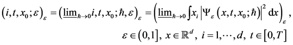(1.2)

and limiting quantum trajectories, such that

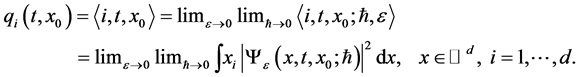(1.3)

if limit in LHS of Equation (1.3) exists.

The physical interpretation of these asymptotic given below, shows that the answer is “yes” for the limiting quantum trajectories with localized initial data.

Note that an axiom of quantum measurement is: if the particle is in some state that the probability of getting a result at instant with an accuracy of will be given by

. (1.4)

We rewrite now Equation (1.4) of the form

(1.5)

We define well localized limiting quantum trajectories,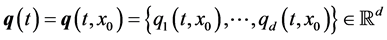

, such that:

(1.6)

and well localized limiting quantum trajectories, , such that:

(1.7)

if limit in LHS of Equation (1.7) exists.

2. Colombeau Solutions of the Schrödinger Equation and Corresponding Path Integral Representation

Let be a complex infinite dimensional separable Hilbert space, with inner product and norm.

Let us consider Schrödinger equation:

, (2.1)

. (2.2)

Here operator is essentially self-adjoint, is the closure of.

Theorem 2.1. [19] [20] . Assume that: (1), (2) is continuous and

. Then corresponding solution of the Schrödinger Equations (2.1)-(2.2) exist and can be represented via formulae

, (2.3)

where we have set and

, (2.4)

where, Let be a trajectory; that is, a function from to with and set

,. We rewrite Equation (2.3) for a future application symbolically for short of the following form

, (2.5)

where we have set 1) and 2) that is, a

, (2.6)

Trotter and Kato well known classical results give a precise meaning to the Feynman integral when the potential is sufficiently regular [18] [19] . However if potential is a non-regular this is well known problem to represent solution of the Schrödinger Equations (2.1)-(2.2) via formulae (2.3), see [19] .

We avoided this difficulty using contemporary Colombeau framework [16] - [18] . Using replacement

, , we obtain from potential regularized

Potential, such that and

1),

. (2.7)

Here is Colombeau algebra of Colombeau generalized functions [16] - [18] .

Finally we obtain regularized Schrödinger equation of Colombeau form [21] - [24] :

, (2.8)

. (2.9)

Using the inequality (2.7) Theorem 2.1 asserts again that corresponding solution of the Schrödinger Equations (2.8)-(2.9) exist and can be represented via formulae:

, (2.10)

where we have set and

, (2.11)

where we have set.

We rewrite Equation (2.10) for a future application symbolically of the following form

, (2.12)

or of the following form

. (2.13)

For the limit in RHS of (2.12) and (2.13) we will be used canonical path integral notation

, (2.14)

where.

Substitution into RHS of the Equation (2.10) gives

.

(2.15)

We rewrite Equation (2.15) for a future application symbolically of the following form

, (2.16)

or of the following form

. (2.17)

For the limit in RHS of (2.16) and (2.17) we will be used following path integral notation

. (2.18)

Let us consider now regularized oscillatory integral

. (2.19)

Lemma 2.1. (Localization Principle [25] [26] ) Let be a domain in and be a smooth function of compact support, , be a real valued smooth function without stationary points in, i.e. for. Let be a differential operator

. (2.20)

Then there exist such that

. (2.21)

Lemma 2.2. (Generalized Localization Principle) Let be a domain in and be a real valued smooth function without stationary points in, i.e. for and let be infinite sequence:

. (2.22)

Then there exist infinite sequence, such that

.

Proof. Equality (2.23) immediately follows from (2.21).

Remark 2.1. From Lemma 2.2 follows that stationary phase approximation is not a valid asymptotic approximation in the limit for a path-integral (2.14) and (2.18).

3. Exact Quasi-Classical Asymptotic Beyond Maslov Canonical Operator

Theorem 3.1. Let us consider Cauchy problem (2.8) with initial data is given via formula

, (3.1)

where and.

1) We assume now that: a), b) and c) function is a polynomial on variable, i.e.

. (3.2)

2) Let be the solution of the boundary problem

, (3.3)

. (3.4)

Here, ,

. (3.5)

3) Let be the master action given via formula

, (3.6)

where master Lagrangian are

, (3.7)

. (3.8)

Let be solution of the linear system of the algebraic equations

. (3.9)

4) Let be solution of the linear system of the algebraic equations

. (3.10)

Assume that: for a given values of the parameters the point is not a focal point on a corresponding trajectory is given by corresponding solution of the boundary problem (3.3). Then for the limiting quantum average given via formulae (1.1) the inequalities is satisfied:

. (3.11)

Thus one can to calculate the limiting quantum trajectory corresponding to potential by using transcendental master equation

. (3.12)

Proof. From inequality (A.15) and Theorem A1, using inequalities (A.53.a) and (A.53.b) we obtain

, (3.13)

where

, (3.14)

. (3.15)

We note that

, (3.16)

where

(3.17)

(3.18)

and

(3.19)

. (3.20)

From Equation (3.18) one obtain

, (3.21)

where

, (3.22)

. (3.23)

Let us calculate now path integral and path integral, using stationary phase approximation. From Equation (A.23) follows directly that action coincide with master action is given via formulae (3.6)-(3.8) and therefore from Equation (3.22) and Equation (3.23) one obtain

(3.24)

and

(3.25)

From Equation (3.17) and Equation (3.24) we obtain

. (3.26)

Substitution Equation (3.25) into Equation (3.26) gives

. (3.26')

Similarly one obtain

. (3.27)

Let us calculate now integral and integral using stationary phase approximation. Let be the stationary point of master action and therefore Equation (3.9) is satisfied. Having applied stationary phase approximation one obtain

, (3.28)

. (3.29)

Substitution Equations (3.28)-(3.29) into Equation (3.21) gives

(3.30)

Substitution Equation (3.30) into Equation (3.16) gives

(3.31)

Similarly one obtain

(3.32)

Therefore

. (3.33)

Substitution Equation (3.1) into Equation (3.33) gives

. (3.34)

Let us calculate now integral (3.34) using Laplace’s approximation. It is easy to see that corresponding stationary point is the solution of the linear system of the algebraic Equation (3.10). Therefore finally we obtain

. (3.35)

Substitution Equation (3.35) into inequality (3.13) gives the inequality (3.11). The inequality (3.11) completed the proof.

4. Quantum Anharmonic Oscillator with a Cubic Potential Supplemented by Additive Sinusoidal Driving

In this subsection we calculate exact quasi-classical asymptotic for quantum anharmonic oscillator with a cubic potential supplemented by additive sinusoidal driving. Using Theorem 3.1 we obtain corresponding limiting quantum trajectories given via Equation (1.3).

Let us consider quantum anharmonic oscillator with a cubic potential

. (4.1)

Supplemented by an additive sinusoidal driving. Thus

. (4.2)

The corresponding master Lagrangian given by (3.7), are

. (4.3)

We assume now that: and rewrite (4.3) of the form

. (4.4)

where and.

The corresponding master action given by Equation (3.6), are

(4.5)

The linear system of the algebraic Equation (3.9) are

(4.6)

Therefore

. (4.7)

The linear system of the algebraic Equation (3.10) are

. (4.8)

Therefore the solution of the linear system of the algebraic Equation (3.10) are

. (4.9)

Transcendental master Equation (3.11) are

(4.10)

Finally from Equation (4.10) one obtain

. (4.11)

where.

Numerical Examples

Example 1 (in Figure 1 and Figure 2)., , , , , ,.

5. Comparison Exact Quasi-Classical Asymptotic with Stationary-Point Approximation

We set now. Let us consider now path integral (2.14) with given via formula

. (5.1)

Note that for corresponding propagator the time discretized path-integral representation are:

, (5.2)

where are:

. (5.3)

Here the initial- and end-points are fixed by the prescribed and by the additional constraint.

Let us calculate now integral (5.2) using stationary-point approximation. Denoting an critical points of the discrete-time action (5.3) by it follows that satisfies the critical point conditions are

(5.4)

for, supplemented by the prescribed boundary conditions for, ,.

From Equation (5.2) in the limit using formally stationary-point approximation one obtain

. (5.5)

Here the pre-factor is given via N-dimensional Gaussian integral of the canonical form as

. (5.6)

The Gaussian integral in (5.6) is given via canonical formula

. (5.7)

Here denote the determinant of an matrix with elements.

Let us consider now Cauchy problem (2.8) with initial data is given via formula

.

Note that for corresponding Colombeau solution given via path-integral (2.14) the time discretized path-integral representation are

(5.8)

Let us calculate now integrals in RHS of Equation (5.8) using stationary-point approximation. Corresponding critical point conditions are

. (5.9)

From (5.8) we obtain

. (5.10)

. (5.11)

Let as denote the critical point for which the critical point conditions (5.4) are

. (5.12)

Therefore the time discretized path-integral representation of the Colombeau quantum averages given by Equation (1.1) are

(5.13)

where, ,. Let us calculate now integrals in RHS of Equation (5.13) using stationary- point approximation. Corresponding critical point conditions are

, (5.14)

. (5.15)

Here can be calculated using linear recursion (5.12) with initial data.

From Equations (5.13)-(5.14) one obtain

, (5.16)

and. (5.17)

As demonstrated in [24] the determinant appearing in (5.11) can be calculated using second order linear recursion:

(5.18)

with initial data, (5.19)

from which the pre-factor in (5.16) follows as

. (5.20)

In the limit from critical point conditions (5.12) and (5.14) one obtain

. (5.21)

In the limit from a second order linear recursion (5.18) one obtain the second order linear differential equation

(5.22)

with initial data

. (5.23)

By integration Equation (5.22) one obtain the first order linear differential equation

. (5.24)

In the limit from Equation (5.16), Equations (5.20)-(5.21) and Equation (5.24) one obtain

. (5.25)

We set now in Equation (5.1)

. (5.26)

Corresponding differential master equation are

. (5.27)

From Equation (5.27) one obtain that corresponding transcend dental master equation are

(5.28)

Numerical Examples

Comparison of the: 1) classical dynamics calculated by using Equation (5.1) (red curve), 2) limiting quantum trajectory calculated by using master equation Equation (5.28) (blue curve) and 3) limiting quantum trajectory calculated by using stationary-point approximation given by Equation (5.25) (green curve) (in Figure 3 and Figure 4).

6. Conclusions

We pointed out that there existed limiting quantum trajectories given via Equation (1.3) with a jump. Such jump does not depend on any single measurement of particle position at instant and is obtained without any reference to a phenomenological master-equation in Lindblad’s form.

An axiom of quantum mechanics is that we cannot predict the result of any single measurement of an observable of a quantum mechanical system in a superposition of eigenstates. However we can predict the result of any single measurement of particle position at instant with a probability if valid the condition:, where is given by Equation (1.5).

Acknowledgements

A reviewer provided important clarification.

Cite this paper

Jaykov Foukzon,Alex Potapov,Stanislav Podosenov, (2015) Exact Quasi-Classical Asymptotic beyond Maslov Canonical Operator and Quantum Jumps Nature. Journal of Applied Mathematics and Physics,03,584-607. doi: 10.4236/jamp.2015.35072

References

Appendix

Let us consider now regularized Feynman-Colombeau propagator given by Feynman path integral:

, (A.1)

where,

, (A.2)

, (A.3)

(A.4)

(A.5)

, (A.6)

,

, (A.7)

. (A.8)

Here:1), and 2) for each path q(t) such that,

, , where is a given function, operator are

. (A.9)

3) is a positive Feynman “measure”.

Therefore regularized Colombeau solution of the Schrödinger equation corresponding to regularized propagator (A.1) are

(A.10)

Here. (A.11)

Let us consider now regularized quantum average

. (A.12)

From (A.5) and (A.12) one obtain

(A.13)

From Equations (A.5)-(A.13) one obtain

(A.14)

Using replacement, into RHS of the Equation (A.9) one obtain

(A.15)

Here

(A.16)

And

(A.17)

(A.18)

Let us rewrite a function in the following equivalent form:

, (A.19)

, (A.20)

, (A.21)

where, , ,.

Let use valuate now path integral given via Equation (A.17). Substitution Equation (A.19) into RHS of the Equation (A.17) gives

,

(A.22.a)

,

(A.22.b)

where

, (A.23)

, (A.24)

(A.25.a)

(A.25.b)

(A.26.a)

(A.26.b)

Let us evaluate now n-dimensional path integral:

(A.27)

From Equation (A.27) one obtain the inequality

(A.28)

From In Equation (A.28) one obtain the inequality

(A.29)

where

, (A.30)

. (A.31)

Using replacement, , into RHS of the Equation (A.31) one obtain

(A.32)

, , , see Equation (3.1) and

, (A.33)

. (A.34)

. (A.35)

From (A.29)-(A.35) one obtain

(A.36)

. (A.37)

Proposition A.1. [27] [28] Let be a double sequence. Let.

Then the iterated limit: exist and equal to if and only if exists for each.

Proposition A.2. Let, where is given via Eq-

uation (A.25) and let, where is given via Equa-

tion (A.26). Then

1)

2),

3),

4)

5),

6).

Here

,

.

Proof (I) Let us to choose an sequence such that

1) and

2).

We note that from (ii) follows that: perturbative expansion

vanishes in the limit. From (A.36) and Schwarz’s inequality using Proposition A.1, one obtain

(A.38)

Let us to choose now an subsequence such that the limit:

exist and, (A.39)

From (A.39) and Proposition A.1 one obtain

. (A.40)

From (A.39), (A.40) and (A.38) one obtain

(A.41)

The inequality (A.41) completed the proof of the statement (1).

(II) Let us estimate now n-dimensional path integral

(A.42)

From Equation (A.42) one obtain the inequality

(A.43)

where

. (A.44)

Using replacement, , into RHS of the Equation (A.44) one obtain

(A.45)

, , , see Equation (3.1) and

, (A.46)

. (A.47)

. (A.48)

From (A.43)-(A.48) one obtain

. (A.49)

Let us to choose an sequence such that

1) and

2).

We note that from 2) follows that: perturbative expansion

,

Vanishes in the limit. From (A.49) one obtain

. (A.50)

Let us to choose now an subsequence such that the limit:

exist and (A.51)

From (A.51) and Proposition A.1 one obtain

. (A.52)

From (A.50), (A.51) and (A.52) one obtain

Proof of the statements (3)-(6) is similarly to the proof of the statements (1)-(2).

Theorem A.1. Let, ,

where is given via Equations (A.22a)-(A.22b). Then

(A.53.a)

(A.53.b)

Here

, (A.54)

. (A.55)

Proof. We remain that

. (A.56)

From Equation (A.56) we obtain

. (A.57)

Let us to choose now an sequences, , such that:

1),

2), (A.58)

3) (A.59)

Therefore from inequality (A.57), Equation (A.58) and inequality (A.59) we obtain

(A.60)

References

- 1. Vijay, R., Slichter, D.H. and Siddiqi, I. (2011) Observation of Quantum Jumps in a Superconducting Artificial Atom. Physical Review Letters, 106, Article ID: 110502.
http://dx.doi.org/10.1103/PhysRevLett.106.110502 - 2. Peil, S. and Gabrielse, G. (1999) Observing the Quantum Limit of an Electron Cyclotron: QND Measurements of Quantum Jumps between Fock States. Physical Review Letters, 83, 1287-1290.
- 3. Sauter, T., Neuhauser, W., Blatt, R. and Toschek, P.E. (1986) Observation of Quantum Jumps. Physical Review Letters, 57, 1696-1698.
http://dx.doi.org/10.1103/PhysRevLett.57.1696 - 4. Bergquist, J.C., Hulet, R.G., Itano, W.M. and Wineland, D.J. (1986) Observation of Quantum Jumps in a Single Atom. Physical Review Letters, 57, 1699-1702.
http://dx.doi.org/10.1103/PhysRevLett.57.1699 - 5. Bohr, N. (1913) On the Constitution of Atoms and Molecules. Philosophical Magazine, 26, 1-25.
http://dx.doi.org/10.1080/14786441308634955 - 6. Dum, R., Zoller, P. and Ritsch, H. (1992) Monte Carlo Simulation of the Atomic Master Equation for Spontaneous Emission. Physical Review A, 45, 4879.
http://dx.doi.org/10.1103/PhysRevA.45.4879 - 7. Dalibard, J., Castin, Y. and Mølmer, K. (1992) Wave-Function Approach to Dissipative Processes in Quantum Optics. Physical Review Letters, 68, 580.
- 8. Gatarek, D. (1991) Continuous Quantum Jumps and Infinite-Dimensional Stochastic Equations. Journal of Mathematical Physics, 32, 2152-2157.
- 9. Molmer, K., Castin, Y. and Dalibard, J. (1993) Monte Carlo Wave-Function Method in Quantum Optics. Journal of the Optical Society of America B, 10, 524-538.
http://dx.doi.org/10.1364/JOSAB.10.000524 - 10. Gardiner, C.W., Parkins, A.S. and Zoller, P. (1992) Wave-Function Quantum Stochastic Differential Equations and Quantum-Jump Simulation Methods. Physical Review A, 46, 4363-4381.
- 11. Vogt, N., Jeske, J. and Cole, J.H. (2013) Stochastic Bloch-Redfield Theory: Quantum Jumps in a Solid-Stateenvironment. Physical Review B, 88, Article ID: 174514.
- 12. Reiner, J.E., Wiseman, H.M. and Mabuchi, H. (2003) Quantum Jumps between Dressed States: A Proposed Cavity-QED Test Using Feedback. Physical Review A, 67, Article ID: 042106.
http://dx.doi.org/10.1103/PhysRevA.67.042106 - 13. Berkeland, D.J., Raymondson, D.A. and Tassin, V.M. (2004) Tests for Non-Randomness in Quantum Jumps. Physical Review A, 69, Article ID: 052103.
- 14. Wiseman, H.M. and Milburn, G.J. (1993) Interpretation of Quantum Jump and Diffusion Processes Illustrated on the Bloch Sphere. Physical Review A, 47, 1652-1666.
http://dx.doi.org/10.1103/PhysRevA.47.1652 - 15. Wiseman, H.M. and Toombes, G.E. (1999) Quantum Jumps in a Two-Level Atom: Simple Theories versus Quantum Trajectories. Physical Review A, 60, 2474.
http://dx.doi.org/10.1103/PhysRevA.60.2474 - 16. Stojanovic, M. (2008) Regularization for Heat Kernel in Nonlinear Parabolic Equations. Taiwanese Journal of Mathematics, 12, 63-87.
http://www.tjm.nsysu.edu.tw/ - 17. Garetto, C. (2008) Fundamental Solutions in the Colombeau Framework: Applications to Solvability and Regularity Theory. Acta Applicandae Mathematicae, 102, 281-318.
http://dx.doi.org/10.1007/s10440-008-9220-8 - 18. Foukzon, J., Potapov, A.A. and Podosenov, S.A. (2011) Exact Quasiclassical Asymptotics beyond Maslov Canonical Operator. International Journal of Recent advances in Physics, 3.
http://arxiv.org/abs/1110.0098 - 19. Feynman, E.N. (1964) Integrals and the Schrodinger Equation. Journal of Mathematical Physics, 5, 332-343.
http://dx.doi.org/10.1063/1.1704124 - 20. Maslov, V.P. (1976) Complex Markov Cheins and Continual Feynman Integral. Nauka, Moskov.
- 21. Apostol, T.M. (1974) Mathematical Analysis. 2nd Edition, Addison-Wesley, Boston.
- 22. Chen, W.W.L. (2003) Fundamentals of Analysis. Published by Chen, W.W.L. via Internet.
- 23. Gupta, S.L. and Rani, N. (1998) Principles of Real Analysis. Vikas Puplishing House, New Delhi.
- 24. Lehmann, J., Reimann, P. and Hanggi, P. (2000) Surmounting Oscillating Barriers: Path-Integral Approach for Weak Noise. Physical Review E, 62, 6282.
http://dx.doi.org/10.1103/PhysRevE.62.6282 - 25. Fedoryuk, M.V. (1977) The Method of Steepest Descent. Moscow. (In Russian)
- 26. Fedoryuk, M.V. (1989) Asymptotic Methods in Analysis. Encyclopaedia of Mathematical Sciences, 13, 83-191.
http://dx.doi.org/10.1007/978-3-642-61310-4_2 - 27. Shun, Z. and McCullagh, P. (1995) Laplace Approximation of High Dimensional Integrals. Journal of the Royal Statistical Society: Series B (Methodological), 57, 749-760.
- 28. Foukzon, J. (2014) Strong Large Deviations Principles of Non-Freidlin-Wentzell Type-Optimal Control Problem with Imperfect Information—Jumps Phenomena in Financial Markets. Communications in Applied Sciences, 2, 230-363.