Open Journal of Forestry
Vol.05 No.04(2015), Article ID:55842,17 pages
10.4236/ojf.2015.54041
Estimation of Tree Biomass, Carbon Stocks, and Error Propagation in Mecrusse Woodlands
Tarquinio Mateus Magalhães1,2*, Thomas Seifert2
1Departamento de Engenharia Florestal, Universidade Eduardo Mondlane, Maputo, Mozambique
2Department of Forest and Wood Science, University of Stellenbosch, Stellenbosch, South Africa
Email: *tarqmag@yahoo.com.br
Copyright © 2015 by authors and Scientific Research Publishing Inc.
This work is licensed under the Creative Commons Attribution International License (CC BY).
http://creativecommons.org/licenses/by/4.0/


Received 30 March 2015; accepted 17 April 2015; published 21 April 2015
ABSTRACT
We performed a biomass inventory using two-phase sampling to estimate biomass and carbon stocks for mecrusse woodlands and to quantify errors in the estimates. The first sampling phase involved measurement of auxiliary variables of living Androstachys johnsonii trees; in the second phase, we performed destructive biomass measurements on a randomly selected subset of trees from the first phase. The second-phase data were used to fit regression models to estimate below and aboveground biomass. These models were then applied to the first-phase data to estimate biomass stock. The estimated forest biomass and carbon stocks were 167.05 and 82.73 Mg・ha−1, respectively. The percent error resulting from plot selection and allometric equations for whole tree biomass stock was 4.55% and 1.53%, respectively, yielding a total error of 4.80%. Among individual variables in the first sampling phase, diameter at breast height (DBH) measurement was the largest source of error, and tree-height estimates contributed substantially to the error. Almost none of the error was attributable to plot variability. For the second sampling phase, DBH measurements were the largest source of error, followed by height measurements and stem-wood density estimates. Of the total error (as total variance) of the sampling process, 90% was attributed to plot selection and 10% to the allometric biomass model. The total error of our measurements was very low, which indicated that the two-phase sampling approach and sample size were effective for capturing and predicting biomass of this forest type.
Keywords:
Aboveground Production, Additivity, Androstachys johnsonii Prain, Belowground Carbon Allocation, Error Margins, Root Growth

1. Introduction
Mecrusse is a forest type dominated by Androstachys johnsonii Prain, which generally occupies between 80% and 100% of the canopy (Mantilla & Timane, 2005) . A. johnsonii (family Euphorbiaceae) is native to Africa and Madagascar and is the sole member of genus Androstachys; today, mecrusse forest is primarily found in Mozambique (Cardoso, 1963) .
Mecrusse is an important woodland. Besides being restricted to Mozambique (Cardoso, 1963) , it has important socio-economic value to local communities, which use stakes of A. johnsonii in the construction of homes, shelters, and furniture. At the global scale, mecrusse forest forms part of the woodland belt that stretches over large portions of southern Africa and is reported to be a tipping point in regional ecological and socio-economic development (Leadley et al., 2010) . Carbon sequestration in tree biomass is a key ecosystem service provided by woodlands. However, to date, no estimates of biomass or carbon stocks are available for these woodlands despite the relevance of this vegetation type in Mozambique.
Estimates of biomass stock are important for predicting carbon fluxes and stocks, assessing nutrient cycling and fluxes, determining potential wood energy, and for policy making. The errors associated with biomass estimates must be known for the derived predictions and policies to be reliable. However, the error is rarely evaluated carefully in biomass studies (Chave et al., 2004) . Many studies that estimate biomass stock employ a two- phase sampling design; most of these studies found that the error due to second phase (error due to allometric equations) to be larger than that of the first phase (error due to plot selection) (Samalka, 2007; Chave et al., 2004; Molto et al., 2012 ). The error of estimates from two-phase sampling has two main components, one associated with each phase (Cunia, 1986a; Cunia, 1990) . Moreover, each variable measured in each sampling phase contributes to the error of that phase. The objective of this study was to estimate the above and belowground biomass and carbon stocks of mecrusse woodlands and to quantify the errors in those estimates.
2. Material and Methods
2.1. Study Area
In Mozambique, mecrusse woodlands are mainly found in Inhanbane and Gaza provinces, in Massangena, Chicualacuala, Mabalane, Chigubo, Guijá, Mabote, Funhalouro, Panda, Mandlakaze, and Chibuto districts. The easternmost mecrusse forest patches, located in Mabote, Funhalouro, Panda, Mandlakaze, and Chibuto districts, were defined as the study area. The study area comprised 4,502,828 ha (Dinageca, 1997) , of which 226,013 ha (5%) were mecrusse woodlands. The physical and natural conditions for each district of the study area are summarized in Table 1.

Table 1. Physical and natural conditions of the study area.
Sources: Dinageca (1997), Mae (2005a-e) , and FAO (2003) .
2.2. Sampling and Data Collection
The first sampling phase involved the selection of a large number of trees (3574 trees) in randomly located plots for measurement of diameter at breast height (DBH) and total tree height, which were expected to be correlated with component and whole tree biomass. The second phase involved the selection of a subset of trees from the first phase for destructive measurement of biomass, along with the variables of the first phase. Simple random sampling was used in both phases.
2.2.1. First Phase: Plot-Level Sampling and Measurements
We established 23 randomly located circular plots (20-m radius) in the study area; randomness was achieved using Hawth’s Tools in ArcGIS 9.3 (ESRI, 2009) . The plots were located using a GPS and maps and were demarcated on the ground using a Vertex IV hypsometer and a 360˚ transponder. DBH and total height were measured for all trees with DBH ≥ 5 cm in each plot.
2.2.2. Second Phase: Tree-Level Sampling and Measurements
Within each of the 23 plots, 2 to 6 trees (n = 93 total) were selected in proportion to the frequency of five diameter classes for destructive biomass sampling; diameter classes with >5 trees were included. Each tree was felled and divided into the following components: 1) root system, 2) stem wood, 3) stem bark, and 4) crown. The root system was completely excavated, including the fine roots. Tree components were sampled and the dry weights estimated as follows.
1) Root System
The stump height was predefined as being 20 cm for all trees and considered as part of the taproot, as recommended by Parresol (2001) and because in larger A. johnsonii trees this height (20 cm) is affected by root buttress; thus, the root collar was also considered part of the taproot. The root system was divided into 3 sub-com- ponents: fine lateral roots, coarse lateral roots and taproot. Lateral roots with diameters at the insertion point on the taproot < 5 cm were considered as fine roots and those with diameters ≥ 5 cm were considered as coarse roots.
First, the root system was partially excavated to the first node, using hoes, shovels, and picks, to expose the primary lateral roots (Figure 1(a) and Figure 1(b)). The primary lateral roots were numbered and separated from the taproot with a chainsaw (Figures 1(a)-(c)) and removed from the soil, one by one. This procedure was repeated in the subsequent nodes until all primary roots were removed from the taproot and from the soil. Finally, the taproot was excavated and removed (Figure 1(c) and Figure 1(d)). The complete removal of the root system was relatively easy because 90% of the lateral roots of A. johnsonii are located in the first node, which is

Figure 1. Separation of lateral roots from the taproot ((a), (b)), and removal of the taproot including the root collar and the stump ((c), (d)).
located close to ground level (Figures 1(a)-(c)); the lateral roots grow horizontally to the ground level, do not grow downwards; and because the taproots had, at most, only 4 nodes and at least 1 node (at ground level).
Fresh weight was obtained for the taproot, each coarse lateral root and for all fine lateral roots. A sample was taken from each sub-component, fresh weighed, marked, packed in a bag, and taken to the laboratory for oven drying. For the taproot, the samples were two discs, one taken immediately below the ground level and another from the middle of the taproot. For the coarse lateral roots, two discs were also taken, one from the insertion point on the taproot and another from the middle of it. For fine roots the sample was 5% to 10% of the fresh weight of all fine lateral roots. Oven drying of all samples was done at 105˚C to constant weight, hereafter, referred to as dry weight.
2) Stem Wood and Stem Bark
Felled trees were scaled up to a 2.5 cm top diameter. The stem was defined as the length of the trunk from the stump to the height that corresponded to 2.5 cm diameter. The remainder (from the height corresponding to 2.5 cm diameter to the tip of the tree) was considered a fine branch. The stem was divided into sections, the first with 1.1 m length, the second with 1.7 m, and the remaining with 3 m, except the last, which length depended on the length of the stem. Discs were removed at the bottom and top of the first section, and on the top of the remaining sections; i.e.: discs were removed at heights of 0.2 m (stump height), 1.3 m (breast height), 3 m, and the successive discs were removed at intervals of 3 m to the top of the stem, and their fresh weights measured using a digital scale.
Diameters over and under bark were taken from the discs in the North-South direction (previously marked on the standing tree) with the help of a ruler. The volumes over and under the bark of the stem were obtained by summing up the volumes of each section calculated using Smalian’s formula (de Gier, 1992; Husch et al., 2003) . Bark volume was obtained from the difference between volume over bark and volume under bark.
The discs were dipped in drums filled with water for its saturation (3 to 4 months) and subsequent determination of the saturated volume and basic density. The saturated volume of the discs was obtained based on the water displacement method (Brasil et al., 1994) using Archimedes’ principle. This procedure was done twice: before and after debarking; hence, we obtained saturated volume under and over the bark.
Wood discs and respective barks were oven dried at 105˚C to constant weight. Basic density was obtained by dividing the oven dry weight of the discs (with and without bark) by the relevant saturated wood volume (de Gier, 1992; Bunster, 2006) . Therefore, two distinct basic densities were calculated: 1) basic density of the discs with bark and 2) basic density of the discs without bark.
We estimated the basic density at point of geometric centroid of each section using the regression function of density over height (Seifert & Seifert, 2014) . This density value was taken as representative of each section (Seifert & Seifert, 2014) .
3) Crown
The crown was divided into two sub-components: branches and foliage. Primary branches, originating from the stem, were classified in two categories: primary branches with diameters at the insertion point on the stem ≥ 2.5 cm were classified as large branches, and those with diameters < 2.5 cm were classified as fine branches.
Large branches were sampled similarly to coarse roots, and fine branches and foliage were sampled similarly to fine roots. All the leaves from each tree were collected and fresh weighed together and a sample taken for oven drying. The sub-components branches and foliage were not treated as separated components because in the preliminary analysis the weight of the foliage did not show significant variation with DBH, total tree height (H), and live crown length (LCL); exhibiting, therefore, poor fits.
4) Tree Component Dry Weights, and Carbon Concentration
Dry weights of coarse and fine roots, large and fine branches, and foliage were obtained from the “fresh weight/oven dry weight” ratio of the respective samples by multiplying it by the relevant sub-component total fresh weight. Dry weights of the root system and crown were obtained by summing up the relevant sub-com- ponents’ dry weights. Dry weights of each stem (with and without bark) were obtained by multiplying respective average densities by relevant stem volumes. The dry weight of the stem bark was obtained from the difference between the dry weights of stem and stem wood. Finally, the total tree biomass was obtained by adding the component dry weights.
A subsample (n = 17 trees) was randomly selected from the 93 harvested trees (one to two trees per diameter class and location) for carbon analysis. Five samples were randomly selected from each of these 17 trees, from each of the components: roots, leaves, branches, bark, and stem. The samples were pooled and milled together by component to form a composite sample. Carbon concentration in the composite samples was measured using a TruSpec Micro analyser (LECO Corp) at the Central Analytical Facilities, Stellenbosch University (Stellenbosch, South Africa). The average carbon content of the crown was obtained from the average values for branches and foliage. Carbon concentrations for each tree component, with standard deviation (SD) and coefficient of variation (CV, in percentage), are presented in Table 2.
2.3. Biomass Models
Biomass estimation typically requires estimation of tree components and total tree biomass (Seifert & Seifert, 2014) . To ensure the additivity of component biomass estimates into total tree biomass, component and total biomass models were fitted using the same regressors (Parresol, 1999; Goicoa et al., 2011) (conventional method of enforcing additivity). For this, first the best tree component and total tree biomass equations were selected by running various possible linear regressions on combinations of the independent variables (DBH, H, and LCL) and evaluating them using the following goodness of fit statistics: coefficient of determination (R2), standard deviation of the residuals (Sy.x) and CV of the residuals, mean residual (MR), and graphical analysis of the residuals. The computation and interpretation of these fit statistics were previously described by Meyer (1941); Gadow & Hui (1999), Ruiz-Peinado et al. (2011) , and Goicoa et al. (2011) .
Among the different model forms tested, the model form  was the best for three components (root system, stem wood, and stem bark) and for the total tree biomass, and the second best for crown biomass. Therefore, to allow all three components and total tree models to have the same regressors, and thus achieve additivity, this model form was generalized for all tree component and total tree models.
Linear weighted least squares were used to address heteroscedasticity. The weight functions were obtained by iteratively finding the optimal weight that homogenised the residuals and improved other fit statistics. Among the tested weight functions (1/D, 1/D2, 1/DH, 1/DLCL, 1/D2H, 1/D2LCL), the best weight function was found to be 1/D2H, for all tree components and total tree models. Although, the selected weight function might not be the best one among all possible weights, it is the best approximation found.
Linear models were preferred over nonlinear models because the conventional method of enforcing additivity is only applicable for linear models (Parresol, 1999; Goicoa et al., 2011) and because the procedure of combining the error of the first and second sampling phases (Cunia, 1986a) is limited to biomass regressions estimated by linear weighted least squares (Cunia, 1986a) . Table 3 shows the regression models and their statistics for each tree component and for total biomass.
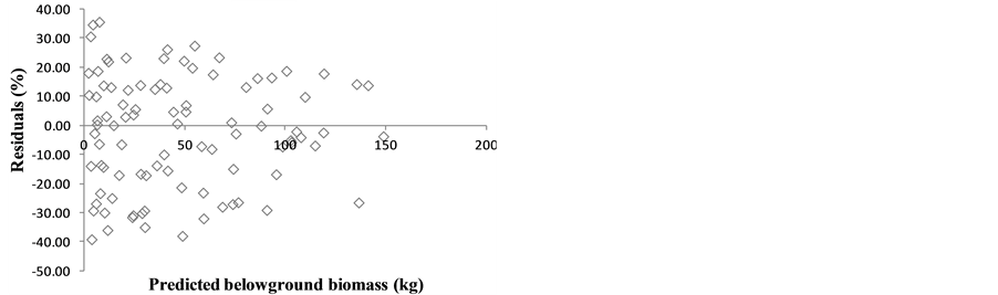
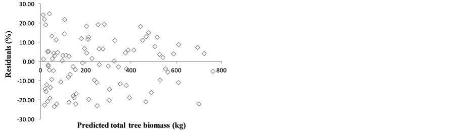
The graphs of the residuals against predicted values for the models in the Table 3 are presented in the Figure 2 and did not show any particular trend or heteroscedasticity.
Table 2. Carbon concentration (%) in each tree component.
Table 3. Parameters (±SE) and fit statistics for the selected models.
Ŷ = tree component biomass (kg); D = diameter at breast height (cm); H = tree height (m); b0 and b1 = regression parameters; SE = standard error of the regression parameters; “*” = significant at α ≥ 5%; “ ” = not significant at any probability level.
 (a)
(a)
 (b) (c)
 (d) (e)
Figure 2. Residuals against predicted biomass for the models in the Table 1.
2.4. Estimation of Biomass and Carbon Stocks
The model equation for component and total tree biomass (Ŷ) was as follows:
 (1)
(1)
where D represents DBH and H represents tree height. The biomass of the kth tree in the hth plot (Ŷhk) estimated by Equation (1) is determined by Equation (2):
 (2)
(2)
The biomass of plot h (Ŷh) is estimated by summing the individual biomass (Ŷhk) values of the nh trees in plot h as follows:
 (3)
(3)
where , and
, and , np = number of plots in the sample, and nh = number of trees in the hth plot. Then, dividing Equation (3) by plot size a gives biomass Ŷ on an area basis:
 (4)
(4)
Denoting  and
and , Equation (4) can be rewritten as:
 (5)
(5)
The biomass stock Ȳ (average biomass per hectare) is estimated by summing the biomass Ŷ of each plot (area basis) and dividing it by the number of plots np:
 (6)
(6)
Now, denoting  and
and , Equation (6) can be rewritten as follows:
 (7)
(7)
where  is the row vector of the regression coefficient of Equation (2) (also referred to as the row vector of the estimates from the second sampling phase), and
  is the column vector of the estimates
from the first phase. As seen in Equation (7), biomass stock is obtained by combining the estimates from the first and second phases.
Equations (2)-(7) were applied to estimate biomass stock of each tree component, whole tree, and diameter class. The carbon stock of each tree component was estimated by multiplying the relevant carbon concentration by biomass stock.
2.5. Error Propagation
Biomass stock (Equation (7)) was estimated by combining the estimates of the first and second phases ( and
and , respectively). Two main sources of error must be accounted for in this calculation, that resulting from
plot-level variability (first sampling phase) and that from the allometric equations (second phase).
Cunia (1965, 1986a, 1986b, 1990) demonstrated that the total variance of the estimated Ȳ (mean biomass per hectare) is given by Equation (8):
 (8)
(8)
where  and
and  are variance components from the first and second sampling phases, respectively;
  and
and  are row and column vectors, respectively, of the regression coefficients;
  and
and  are row and column vectors, respectively, of the estimates from the first phase;
  represents the variance-covari-
ance matrix of vector ; and
; and  represents the variance-covariance matrix of vector
  or of the regression coefficients. In this specific case,
  and
and  are calculated from Equations (9) and (10):
 (9)
(9)
 (10)
(10)
where  = covariance of bi and bj, and
 .
.
The square root of Equation (8) is the total standard error (SE) of Ȳ; the square root of the first component of Equation (8)  is the standard error of the first phase; and the square root of the second component
  is the standard error of the second phase.
In this study, the error of Ȳ is expressed as the percent SE of the first sampling phase (Equation (11)), the second sampling phase (Equation (12)), and both phases combined (Equation (13)):
 (11)
(11)
 (12)
(12)
 (13)
(13)
However, in some cases, the error is expressed as the variance of Ȳ, especially where the proportional influence of a particular source of error needs to be known.
Because carbon stocks are determined by multiplying the carbon concentration by biomass stock, variance of the estimated carbon stock is determined by multiplying the variance of biomass stock by the square of the carbon concentration.
The Monte Carlo error propagation approach was applied to estimate the percent contribution of each variable measurement error to the error of each sampling phase. We determined the contribution of DBH measurement error, height measurement error, and plot variability in the first sampling phase. Plot variability was defined as error resulting from variation in the number of trees per hectare (Sh0). There were numerous sources of error from the second sampling phase; these sources are described below.
Belowground dry weight was determined by summing the dry weights of lateral roots (coarse and fine) and the taproot (Equation (14)). The sources of error in this calculation are the fresh-weight (FW) and moisture content (MC) determinations:
 (14)
(14)
where LR = lateral roots; TR = taproot;  = water weight of lateral roots; and
  = water weight of the taproot. Note that MC is a ratio and varies from 0 to 1.
Equation (14) can be rearranged as:
 (15)
(15)
Dry weight of stem wood was determined by multiplying the estimated mean stem wood basic density (ρsw) by its estimated volume (Equation (16)):

 (16)
(16)
Because the form factor ff and the value  are constants, they do not contribute to error and can be removed to form Equation (17):
 (17)
(17)
Thus, the sources of error in the calculation of stem-wood dry weight are the DBH and height measurements and estimated mean density.
The stem volume obtained by summing the volumes of the constituent stem sections was assumed equal to the volume obtained using form factor; in fact, the mean difference between those two estimates was only 2.3%.
Dry weight of stem bark was calculated as the difference between total stem dry weight (including bark) and dry weight of stem wood (Equation (18)), where ρs is stem basic density (specific gravity):
 (18)
(18)
The sources of errors in Equation (18) include the DBH and height measurements and the estimated mean stem and stem wood basic densities.
Crown dry weight was determined by summing the dry weights of branches and foliage (Eq. 19), with error due to FW and MC determination:
 (19)
(19)
where B = branches; L = leaves;  = water weight of the branches; and
  = water weight of the foliage.
Equation (19) can be rearranged as:
 (20)
(20)
Whole tree dry weight and total error were calculated from the sum of Equations (15), (17), (18) and (20).
The contribution of each phase-1 variable measurement error (DBH, total height, and plot variability) to total phase-1 error was determined using Equation (7) and the phase-1 data; the contribution of error from the second phase was determined from Equations (15), (17), (18) and (20). These calculations were performed using the “propagate” package (Spiess, 2013) in R (R Core Team, 2013) . All statistical analyses were performed at the 95% probability level.
The sources of error accounted for in this study are DBH measurement, total tree height estimation and plot variability for phase-1; and DBH and total tree height measurements, stem and stem wood basic density estimation, determination of moisture content (of foliage, branches, and roots), and measurement of fresh weights (of foliage, branches, and roots) for phase-2. Further research is needed to account for other sources of errors not included here, such as the slop of the terrain, distance between the tree and the hypsometer, diameters at successive heights on the stem, etc.
3. Results
3.1. Biomass and Carbon Stocks
Biomass stock (from Equation (7)) and the corresponding carbon stock (Mg・ha−1), are presented in Table 4 and Table 5, respectively. The whole tree and aboveground biomass stocks were 167 and 134 Mg・ha−1, respectively. Stem wood formed the largest share of biomass for all diameter classes, followed by the crown. The proportional distribution of biomass at the forest scale was as follows: stem wood, 51%; crown, 24%; belowground biomass, 19%; and stem bark, 6%.
The 15 - 20 and 20 - 25 cm diameter classes represented >50% of the total forest biomass stock (Figure 3(a)); however, only ~30% of all trees were in these size classes (Figure 3(b)).
Note that the DBH of A. johnsonii rarely exceeds 35 cm (here, <1% of trees during the first sampling phase); therefore, trees encountered in diameter classes larger than the highest class in Figure 3(b) (25 ≤ DBH < 30) were considered as belonging to this diameter class.
3.2. Error Propagation
Low variance in the estimates of biomass stock indicated that there was a high level of precision in the estimates (Table 6). The largest error was observed for stem bark and crown; the goodness of fit for these components was poorer in the models (smaller R2 and higher CV of the residuals; Table 3), which explained the higher error.
 (a)
(a) (b)
(b)
Figure 3. Proportion of total forest biomass stock (a) and diameter distribution (b) (obtained using phase-1 data) for each diameter class in mecrusse woodlands in the study area.
Table 4. Biomass stock (Mg・ha?1) for each tree component and diameter class.
Table 5. Carbon stock (Mg・ha?1) for each tree component and diameter class.
Table 6. Variance [(Mg・ha−1)2], absolute standard error (Mg・ha−1), and percent standard errors of the estimates of biomass stock for each tree component and sampling phase.
For the crown, the error in the allometric equations (second sampling phase) was equal to the error of plot-level variability (differences in the number of trees per plot in the first sampling phase). In contrast, more of the variance for belowground, stem wood, stem bark, and total biomass was attributable to plot-level variability than to the allometric equations (Table 7).
Subscripts 1 and 2 indicate the first and second sampling phases, respectively; subscript t indicates the total variance or standard error for a given component.
Actual whole tree biomass stock (from 95% CI) was between 151 and 183 Mg・ha−1 (Table 8). Carbon stock (Mg・ha−1) varied from approximately 75 - 91 Mg・ha−1 (Table 9). DBH measurement error contributed close to two-thirds of the error from the first sampling phase, while the tree height measurement error contributed more than one third. Plot-level variability contributes negligibly to the uncertainty (Table 10).
In the second sampling phase (using allometric equations), fresh-weight measurement error accounted for >90% of the total error in biomass calculations. The majority of errors in stem bark and stem wood calculations arose from the errors of basic density estimation and DBH measurements, respectively, while DBH measurement error accounted for most of the error in whole tree biomass calculations (Table 11).
Note that the stem wood basic density estimation is not included as a source of error for the whole tree. The whole tree biomass is obtained by summing Equations (15), (17), (18) and (20); as for the errors. However, by summing Equations (17) and (18) the result is , which excludes stem wood basic density (ρsw). In fact, the stem biomass
  includes both stem wood (Equation (17)) and stem bark biomass (Equation (18)); as for stem density (ρs).
4. Discussion
4.1. Biomass and Carbon Stocks
Our finding that approximately half of total tree biomass and carbon stocks were attributable to stem wood was consistent with the results of Paladinic et al. (2009) for fir-beech and oak forests and Wang et al. (2011) for Abies nephrolepis (Maxim). In Mozambique, A. johnsonii is classified as a first-class commercial species with minimum harvestable diameter of 30 cm (DNFFB, 2002) . Stakes of A. johnsonii used by local communities for construction purposes are generally from trees that are 10 - 15 cm in diameter (Mantilla & Timane, 2005) . This diameter class comprised <20% of the total biomass.
Biomass stock is a function of stem density and DBH, and thus of basal area (see Figure 4, where the diameter classes with the largest proportion of basal area are the same as those with the largest proportion of biomass stock). Biomass stock has been correlated with basal area by many authors (Rai, 1981; Brunig, 1983; Cannell, 1984; Rai & Proctor 1986; Slik et al. 2010) .
In Mozambique, most studies of tree biomass and carbon stocks focus on miombo (Brachystegia spp.) woodlands, which represent 75% of the forest in this country (Sitoe & Ribeiro, 1995) . Existing estimates of biomass and carbon stocks for miombo woodlands are much lower than the estimates obtained here for mecrusse woodlands. Ribeiro et al. (2013) found that the tree biomass and carbon stocks in miombo woodlands of Niassa National Reserve were approximately 59 and 30 Mg・ha−1, respectively. Miombo carbon stocks in Nhambita, Gorongoza District, in Mozambique were estimated as 21.2 Mg・ha−1 for stems and 8.5 Mg・ha−1 for coarse roots (Ryan et al., 2010) .
Low stem density (380 - 400 ha−1) and basal area (7 - 19 m2・ha−1) in miombo (Ribeiro et al., 2002) can explain

Figure 4. Percent basal area distribution for each diameter class in mecrusse woodlands in the study area.
Table 7. Percentage of total error (as variance) attributed to each sampling phase.
Table 8. Biomass stocks and 95% confidence limits.
Table 9. Carbon stocks and 95% confidence limits.
Table 10. Percent contribution of the error of each variable to error of the first sampling phase.
Table 11. Percent contribution of the error of each variable to the error of the second sampling phase.
the lower estimates for biomass and carbon compared to our estimates for mecrusse woodlands (1237 ha−1 and 22 m2・ha−1, respectively). Aboveground biomass estimates by Brown (1997) at the national scale indicated actual and potential biomass stock of 56 and 96 Mg・ha-1, respectively. However, Saatchi et al. (2011) estimated aboveground biomass densities from 51 to 75 Mg・ha−1 for the region in which our study was located. This lower estimate is presumably a result of consideration of other vegetation types (e.g. savannah and thicket) associated with mecrusse woodlands by Saatchi et al. (2011) . Lower values for biomass and carbon stock than those estimated here were also reported in neighbouring countries (Malimbwi et al., 1994; Munishi et al., 2010) .
The default value for carbon content used by the Intergovernmental Panel on Climate Change is 50% (IPCC, 2003) . We compared our measured values with those calculated with this default value and found only slight differences in the estimates (Table 12). However, although the differences were small, these errors would propagate as estimates are scaled up, for example to the stand or forest level.
4.2. Error Propagation
The high level of precision in our biomass estimates was a result of the homogeneity of the tree species and site characteristics (A. johnsonii is the only canopy species in mecrusse forest). Stellingwerf (1994) suggested that the 95% CI should not exceed ±20% of the mean. Brown et al. (1995) reported a total error of 20% for aboveground biomass estimates for Amazonian forests, and this level of precision was considered acceptable. Our 95% CI for estimates of whole tree biomass stock was ±9.6%, which was well within these accepted limits.
We showed that the relatively higher error for stem bark and crown biomass stocks was largely a result of the error in the allometric equations, which were relatively poor models for estimating biomass. These models were poor, presumably because of variation in crown weight among trees with the same DBH and height, which might have been caused by differences in stand density, crown shape, and density of branch wood (Pardé, 1980; Carvalho & Parresol, 2003) , and by variation in stem bark density within and between trees.
Because the overall error was largely attributed to plot selection, the total error could be reduced by increasing the number of sampling plots.
In contrast to our findings, we expected the error due to allometric equations to be larger than that due to sample plot selection, because destructive measurement (phase two) is labour demanding and time consuming and, therefore, more susceptible to errors. However, according to the definition of large sample size suggested by Husch et al. (2003), Stellingwerf (1994), Freese (1962, 1984) and Stauffer (1983) , in which the number of replicates should be >30, our sample for the phase-two measurements (n = 93) was large, which led to lower variance. In contrast, our phase-one sample size (n = 23) might be considered small, yielding relatively large variance values.
Field studies that estimate biomass generally perform destructive sampling on a relatively small number of trees (even in multi-species tropical forests), especially when the roots are included, which leads to higher variance (error) of the second phase. Salis et al. (2006) destructively sampled 10 trees per species to estimate aboveground biomass and obtained wider confidence intervals than the suggested by Stellingwerf (1994) . Wang (2006) and Dias et al. (2006) used sample sizes of 10 and 15 trees per species, respectively, which might not have been sufficient to represent all sources of variation. Malimbwi et al. (1994) performed destructive sampling of 17 trees from 15 species in 10 sample plots in miombo woodland at Kitulangalo Forest Reserve, Tanzania, and obtained a total percent error of 36% for biomass stock. That study examined approximately one tree per species, which (combined with the small number of plots) might have contributed strongly to the large total error.
Samalca (2007) estimated aboveground biomass for a multi-species forest in Indonesia using 143 plots (0.05 ha each, first phase) and destructive sampling of 40 trees (second phase), and found that >60% of total error was
Table 12. Comparison of carbon stock estimates using values estimated with TruSpec Micro analyser (this study) and the IPCC default value (carbon content = 50% of biomass) (IPCC, 2003) .
attributed to allometric equations (second phase). The total variance was attributed to the second phase, where the sample size was relatively small considering the multi-species forest (Samalca 2007) . Chave et al. (2004) and Molto et al. (2012) , using Monte Carlo and Bayesian error propagation approaches, respectively, also found that the most important source of error in biomass estimates for tropical forest was related to allometric equations, in contrast to our findings.
We expected the contribution of DBH measurement error, in both the first and second phase, to be smaller than that of total tree height measurement/estimation as found by some authors (Schmid-Haas et al., 1981; Gertner & Köhl, 1992; Berger et al., 2014) , since DBH is easily and directly measured and thus less susceptible to measurement error than tree height (Loetsch et al., 1973; Machado & Filho 2006; Sanquetta et al., 2006) . The largest contribution of DBH measurement error to the total error of both phases is explained by the higher variability of DBHs compared to total tree height (Table 13). Table 13 shows that the variability (CV) of DBH is, approximately, twice as large as the variability of the total tree height in both phases. Moreover, the quadratic term for DBH in Equations (2), (17), and (18) caused its error to propagate disproportionately (quadratically) to that of the height.
The larger error in height measurements for the first sampling phase compared to the second phase occurred because tree height was measured directly using a tape in the second phase, while height was estimated using a Vertex IV hypsometer in the first phase. In the first phase, the measurements were more susceptible to instrument error, error inherent to the trees, and error caused by the distance between the instrument and the tree.
The relatively higher total percent error for stem bark and crown biomass stock originating in the allometric equations might have been a result of variation in crown weight among trees with the same DBH and height. When the contribution of branches and foliage to error are removed (Table 11), variation in crown weight was seen to be influenced by error in fresh weight of branches, which in turn was a result of variation in branch weight within and between trees. This finding is consistent with findings of Pardé (1980) . The higher error for stem bark in the allometric equations was caused by variations in density.
5. Conclusion
The total tree biomass stock was 167 Mg・ha−1 of which, approximately, 134 Mg・ha−1 was aboveground biomass. Our measurements showed that more than half of the forest biomass and carbon stocks in mecrusse woodlands were contained in stem wood of trees that were 15 - 25 cm in diameter. The total error of our total tree biomass estimate was very low (<5%), which indicated that the two-phase sampling approach and sample size were effective for capturing and predicting biomass of this forest type. Sources of measurement error included the sample plot selection (first phase) and the allometric models (second phase). Measurement errors of DBH and errors in estimates of total height and mean stem density contributed strongly to the total error.
Acknowledgments
This study is funded by the Swedish International Development Cooperation Agency (SIDA). Thanks are extended to Professor Almeida Sitoe for his advices during the preparation of the field work; and to the field and laboratory team involved in felling, excavation, fresh- and dry-weighing of trees and tree samples: Albino Américo Mabjaia, Salomão dos Anjos Baptista, Amélia Saraiva Monguela, João Paulino, Alzido Macamo, Jaime, Bule,
Table 13. Descriptive statistics of DBH and total tree height for both phases.
Adolfo Zunguze, Viriato Chiconele, Murrombe, Paulo Goba, Dinísio Júlio, Gerente Guarinare, Sá Nogueira Lisboa, Francisco Ussivane, Nkassa Amade, Cândida Zita, and José Alfredo Amanze. We would also like to thank the members of local communities, community leaders, and Madeiraarte Forest Concession for the unconditional help. Acknowledges are also due to the anonymous reviewers whose insightful comments and suggestions have improved considerably this paper.
References
- Berger, A., Gschwantner, T., McRoberts, R., & Schadauer, K. (2014). Effects of Measurement Errors on Individual Tree Stem Volume Estimates for the Austrian National Forest Inventory. Forest Science, 60, 14-24. http://dx.doi.org/10.5849/forsci.12-164
- Brasil, M. A. M., Veiga, R. A. A., & Timoni, J. L. (1994). Erros na determinação da densidade básica da madeira. CERNE, 1, 55-57.
- Brown, I. F., Martinelli, L. A., Thomas, W. W., Moreira, M. Z., Ferreira, C. A. C., & Victoria, R. A. (1995). Uncertainty in the Biomass of Amazonian Forests: An Example from Rondônia, Brazil. Forest Ecology and Management, 75, 175-189. http://dx.doi.org/10.1016/0378-1127(94)03512-U
- Brown, S. (1997). Estimating Biomass and Biomass Change of Tropical Forests: A Primer. FAO Forest Paper 134.
- Brunig, E. F. (1983). Structure and Growth. In F. B. Golley (Ed.), Ecosystems of the World 14A, Tropical Rain Forest Ecosystems: Structure and Function (pp. 49-75). New York: Elsevier.
- Bunster, J. (2006) Commercial Timbers of Mozambique, Technological Catalogue. Maputo: Traforest Lda.
- Cannell, M. G. R (1984). Woody Biomass of Forest Stands. Forest Ecology and Management, 8, 299-312. http://dx.doi.org/10.1016/0378-1127(84)90062-8
- Cardoso, G. A. (1963). Madeiras de Moçambique: Androstachys johnsonii. Maputo: Serviços de agricultura e serviços de veterinária.
- Carvalho, J. P., & Parresol, B. R. (2003). Additivity of Tree Biomass Components for Pyrenean oak (Quercus pyrenaica Willd.). Forest Ecology and Management, 179, 269-276. http://dx.doi.org/10.1016/S0378-1127(02)00549-2
- Chave, J., Condic, R., Aguilar, S., Hernandez, A., Lao, S., & Perez, R. (2004). Error Propagation and Scaling for Tropical Forest Biomass Estimates. Philosophical Transactions of the Royal Society B, 309, 409-420. http://dx.doi.org/10.1098/rstb.2003.1425
- Cunia, T. (1965). Some Theory on the Reliability of Volume Estimates in a Forest Inventory Sample. Forest Science, 11, 115-128.
- Cunia, T. (1986a). Error of Forest Inventory Estimates: Its Main Components. In E. H. Wharton, & T. Cunia, (Eds.), Estimat- ing Tree Biomass Regressions and Their Error. NE-GTR-117. (pp. 1-13). Broomall: USDA, Forest Service, Northeastern Forest Experimental Station.
- Cunia, T. (1986b). On the Error of Forest Inventory Estimates: Double Sampling with Regression. In E. H. Wharton, & T. Cunia (Eds.), Estimating Tree Biomass Regressions and Their Error. NE-GTR-117 (pp. 79-87). Broomall: USDA, Forest Service, Northeaster Forest Experimental Station.
- Cunia, T. (1990). Forest Inventory: On the Structure of Error of Estimates. In V. J. LaBau, & T. Cunia (Eds.), State-of-the- Art Methodology of Forest Inventory: A Symposium Proceedings (pp. 169-176). General Technical Report PNW-GTR- 263. Portland: USDA, Forest Service, Pacific Northwest Research Station.
- de Gier, I. A. (1992). Forest Mensuration (Fundamentals). Enschede, Overijssel: International Institute for Aerospace Survey and Earth Sciences (ITC).
- Dias, A. T. C., Mattos, E. A., Vieira, S. A., Azevedo, J. V., & Scarano, F. R. (2006). Aboveground Biomass Stock of Native Woodland on a Brazilian sand Coastal Plain: Estimates Based on the Dominant Tree Species. Forest Ecology and Ma- nagement, 226, 364-367. http://dx.doi.org/10.1016/j.foreco.2006.01.020
- Dinageca (1997). Mapa digital de uso e cobertura de terra. Maputo: CENACARTA.
- DNFFB (2002). Regulamento da lei de florestas e fauna bravia. Maputo: Ministério de Agricultura e Desenvolvimento Rural (MADER).
- ESRI (2009). ArcGis Desktop: Release 9.3. Redlands, CA: Environmental Systems Research Institute.
- FAO (2003). FAO Map of World Soil Resources. Rome: FAO.
- Freese, F. (1962). Elementary Forest Sampling. Washington DC: US Department of Agriculture.
- Freese, F. (1984). Statistics for Land Managers. Edinburgh: Paeony Press.
- Gadow, K. V., & Hui, G. Y. (1999). Modelling Forest Development. Dordrecht: Kluwer Academic Publishers.
- Gertner, G., & Köhl, M. (1992). An Assessment of Some Nonsampling Errors in a National Survey Using an Error Budget. Forest Science, 38, 525-538.
- Goicoa, T., Militino, A. F., & Ugarte, M. D. (2011). Modelling Aboveground Tree Biomass While Achieving the Additivity Property. Environmental and Ecological Statistics, 18, 367-384. http://dx.doi.org/10.1007/s10651-010-0137-9
- Husch, B., Beers, T. W., & Kershaw Jr., J. A. (2003). Forest Mensuration (4th ed.). New York: John Wiley & Sons.
- IPCC (2003). Good Practice Guidance for Land Use, Land-Use Change and Forestry. Hayama: Intergovernmental Panel on Climate Change.
- Leadley, P., Pereira, H. M., Alkemade, R., Fernandez-Manjarrés, J. F., Proença, V., Scharlemann, J. P. W., & Walpole, M. J. (2010). Biodiversity Scenarios: Projections of 21st Century Change in Biodiversity and Associated Ecosystem Services. Technical Series No. 50, Montreal: Secretariat of the Convention on Biological Diversity.
- Loetsch, F., Zöhrer, F., & Haller, K. E. (1973). Forest Inventory, Volume II. München: BLV Verlagsgesellschaft.
- Machado, S. A., & Figueiredo Filho, A. (2006). Dendrometria. Paraná: Editora unicentro.
- Mae (2005a). Perfil do distrito de Chibuto, província de Gaza. Maputo: Mae.
- Mae (2005b). Perfil do distrito de Funhalouro, província de Inhambane. Maputo: Mae.
- Mae (2005c). Perfil do distrito de Mabote, província de Inhambane. Maputo: Mae.
- Mae (2005d). Perfil do distrito de Mandhlakaze, província de Gaza. Maputo: Mae.
- Mae (2005e). Perfil do distrito de Panda, província de Inhambane. Maputo: Mae.
- Malimbwi, R. E., Solberg, B., & Luoga, E. (1994). Estimation of Biomass and Volume in Miombo Woodland at Kitulangalo Forest Reserve, Tanzania. Journal of Tropical Forest Science, 7, 230-242.
- Mantilla, J., & Timane, R. (2005). Orientação para maneio de mecrusse. Maputo: SymfoDesign.
- Meyer, H. A. (1941). A Correction for a Systematic Errors Occurring in the Application of the Logarithmic Volume Equa- tion. Harrisburg, PA: Forestry School Research.
- Molto, Q., Rossi, V., & Blanc, L. (2012). Error Propagation in Biomass Estimation in Tropical Forests. Methods in Ecology and Evolution, 4, 175-183. http://dx.doi.org/10.1111/j.2041-210x.2012.00266.x
- Munishi, P. K. T., Mringi, S., Shirima, D. D., & Linda, S. K. (2010). The Role of the Miombo Woodlands of the Southern Highlands of Tanzania as Carbon Sinks. Journal of Ecology and the Natural Environment, 2, 261-269.
- Paladinic, E., Vuletic, D., Martinic, I., Marjanovic, H., Indir, K., Benko, M., & Novotny, V. (2009). Forest Biomass and Sequestrated Carbon Estimation According to Main Tree Components on the Forest Stand Scale. Periodicum Biologorum, 111, 459-466.
- Pardé, J. D. (1980). Forest Biomass. Forest Abstracts, 41, 343-362.
- Parresol B. R. (1999). Assessing Tree and Stand Biomass: A Review with Examples and Critical Comparisons. Forest Sci- ence, 45, 573-593.
- Parresol, B. R. (2001). Additivity of Nonlinear Biomass Equations. Canadian Journal of Forest Research, 31, 865-878. http://dx.doi.org/10.1139/x00-202
- R Core Team (2013). A Language and Environment for Statistical Computing. Vienna: R Foundation for Statistical Comput- ing.
- Rai, S. N. (1981). Productivity of Tropical Rainforests of Karnataka. Ph.D. Thesis, Bombay: University of Bombay.
- Rai, S. N., & Proctor, J. (1986). Ecological Studies on Four Rainforests in Karnataka, India: I. Environment, Structure, Floristics and Biomass. Journal of Ecology, 74, 439-454. http://dx.doi.org/10.2307/2260266
- Ribeiro, N. S., Matos, C. N., Moura, I. R., Washington-Allen, R. A., & Ribeiro, A. I. (2013). Monitoring Vegetation Dynamics and Carbon Stock Density in Miombo Woodlands. Carbon Balance and Management, 8, 11. http://dx.doi.org/10.1186/1750-0680-8-11
- Ribeiro, N., Sitoe, A. A., Guedes, B. S., & Staiss, C. (2002). Manual de silvicultura tropical. Maputo: Food and Agriculture Organisation of the United Nations.
- Ruiz-Peinado, R., del Rio, M., & Montero, G. (2011). New Models for Estimating the Carbon Sink Capacity of Spanish Softwood Species. Forest Systems, 20, 176-188. http://dx.doi.org/10.5424/fs/2011201-11643
- Ryan, C. M., Williams, M., & Grace, J. (2010). Above- and Belowground Carbon Stocks in a Miombo Woodland Landscape of Mozambique. Biotropica, 43, 423-432.
- Saatchi, S. S., Harris, N. L., Brown, S., Lefsky, M., Mitchard, E. T. A., Salas, W., Zutta, B. R., Buermann, W., Lewis, S. L., Hagen, S., Petrova, S., White, L., Silman, M., & Morel, A. (2011). Benchmark Map of Forest Carbon Stocks in Tropical Regions across Three Continents. Proceedings of the National Academy of Sciences of the United States of America, 108, 9899-9904. http://dx.doi.org/10.1073/pnas.1019576108
- Salis, S. M., Assis, M. A., Mattos, P. P., & Pião, A. C. S. (2006). Estimating the Aboveground Biomass and Wood Volume of Savannah Woodlands in Brazil’s Pantanal Wetlands Based on Allometric Correlations. Forest Ecology and Management, 228, 61-68. http://dx.doi.org/10.1016/j.foreco.2006.02.025
- Samalca, K. I. (2007). Estimation of Forest Biomass and Its Error: A Case in Kalimantan, Indonesia. M.Sc. Thesis, Enschede, Overijssel: International Institute for Geo-Information Science and Earth Observation (ITC).
- Sanquetta, C. R., Watzlawick, L. F., Côrte, A. P. D., & Fernandes, L. A. V. (2006). Inventários florestais: Planejamento e execução. Curitiba: Multi-graphic gráfica e editora.
- Schmid-Haas, P., & Winzeler, K. (1981). Efficient Determination of Volume and Volume Growth. In N. Masahisa (Ed.), Proceedings of Forest Resource Inventory, Growth Models, Management Planning, and Remote Sensing (pp. 231-257). 17th IUFRO World Congress, 6-12 September 1981, Kyoto, Ikarashi, Niigata: Niigata University, Faculty of Agriculture, Laboratory of Forest Mensuration.
- Seifert, T., & Seifert, S. (2014). Modelling and Simulation of Tree Biomass. In T. Seifert (Ed.), Bioenergy from Wood: Sustainable Production in the Tropics. Managing Forest Ecosystems (Vol. 26, pp. 43-65). Berlin: Springer.
- Sitoe, A. A., & Ribeiro, N. S. (1995). Miombo Book Project (Case Study of Mozambique). Maputo: Universidade Eduardo Mondlane (UEM).
- Slik, J. W. F., Aiba, S. I., Brearley, F. Q., Cannon, C. H., Forshed, O., Kitayama, K., Nagamasu, H., Nilus, R., Payne, J., Paoli, G., Poulsen, A. D., Raes, N., Sheil, D., Sidiyasa, K., Suzuki, E., & Valkenburg, J. L. C. H. (2010). Environmental Correlates of Tree Biomass, Basal Area, Wood Specific Gravity and Stem Density Gradients in Borneo’s Tropical Forests. Global Ecology and Biogeography, 19, 50-60. http://dx.doi.org/10.1111/j.1466-8238.2009.00489.x
- Spiess, A. N. (2013). Propagate: Propagation of Uncertainty (R Package Version 1.0-1). Vienna: R Foundation for Statistical Computing.
- Stauffer, H. B. (1983). Some Sample Size Tables for Forest Sampling. British Columbia: Ministry of Forests.
- Stellingwerf, D. A. (1994). Forest Inventory and Remote Sensing. Enschede, Overijssel: International Training Centre for Aerial Survey (ITC).
- Wang, C. K. (2006). Biomass Allometric Equations for 10 Co-Occurring Tree Species in Chinese Temperate Forests. Forest Ecology and Management, 222, 9-16. http://dx.doi.org/10.1016/j.foreco.2005.10.074
- Wang, J., Zhang, C., Xia, F., Zhao, X., Wu, L., & von Gadow, K. (2011). Biomass Structure and Allometry of Abies nephrolepis (Maxim) in Northeast China. Silva Fennica, 45, 211-226. http://dx.doi.org/10.14214/sf.113
NOTES

*Corresponding author.