American Journal of Operations Research
Vol. 2 No. 3 (2012) , Article ID: 22436 , 8 pages DOI:10.4236/ajor.2012.23047
An Efficient Simulated Annealing Approach to the Travelling Tournament Problem
1Department of Industrial Engineering, Sharif University of Technology, Tehran, Iran
2Faculty of Department of Industrial Engineering, Sharif University of Technology, Tehran, Iran
3Department of Computer Engineering, Sharif University of Technology, Tehran, Iran
Email: s_nourollahi@ie.sharif.edu, Eshghi@sharif.edu, shokri@ce.sharif.edu
Received May 28, 2012; revised June 30, 2012; accepted July 12, 2012
Keywords: Travelling Tournament Problem; Simulated Annealing; Graph Coloring; Combinatorial Optimization
ABSTRACT
Scheduling sports leagues has drawn significant attention to itself in recent years, as it involves considerable revenue as well as challenging combinatorial optimization problems. A particular class of these problems is the Traveling Tournament Problem (TTP) which focuses on minimizing the total traveling distance for teams. In this paper, an efficient simulated annealing approach is presented for TTP which applies two simultaneous and disparate models for the problem in order to search the solutions space more effectively. Also, a computationally efficient modified greedy scheme is proposed for constructing a favorable initial solution for the simulated annealing algorithm. Our computational experiments, carried out on standard instances, demonstrate that this approach competes with previous offered methods in quality of found solutions and their computational time.
1. Introduction
Scheduling of sports leagues is considered as an important class of optimization problems, which has received significant attention in recent years, since it has a great impact on the revenue of broadcasting the events on radio or television networks and teams’ costs including travelling expenses. Theoretically, these optimization problems can be solved by trivial mathematical models and algorithms, although in practice leads to disappointing and infeasible computational results by considering the computations time. Accordingly, a great effort has been made to devise improved algorithms resulting in better computational time as much as possible.
This paper studies the Travelling Tournament Problem (TTP) proposed in [1] with the constraint of Double Round-Robin (DRR) scheduling in addition to satisfying specific constraints on the home/away pattern of the games. Travelling Tournament Problem aims to minimize the total amount of distance travelled by teams participating in the tournament. Round-Robins are schedules involving n teams in which every team has to face all other teams in a fixed number of times, say m; accordingly in the case of Double Round-Robin scheduling m is 2. The Round-Robin scheduling, especially Double RoundRobin, is currently applied widely in many major sports tournaments, for instance, Major League Baseball [1] and National Basketball Association [2] leagues of United States and many European national soccer leagues.
This literature proposes a simulated annealing algorithm with some of its features similar to the one proposed by Anagnostopoulos et al. [3] (TTSA), containing certain properties in order to obtain high quality solutions. It exploits graph coloring techniques and further heuristics in order to achieve better computational results rather than TSSA. The data and information used for the purpose of computations and experiments are from the Major League Baseball (MLB) of United States.
2. Literature Review
Scheduling of sports events and competitions mentioned in the literature are organized and have been studied considering two major factors, namely the pattern of home/ away games of the participating teams and the distance these teams have to travel according to the order that is specified by the programmed schedule. Therefore, sports scheduling problems which are addressed in this paper fall into two main categories. The goal of the first category is to minimizes the number of breaks, i.e. two consecutive home game or two consecutive away games, whereas the objective of the second one is to minimize the overall distance which teams have to travel.
Schreuder [4] and De Werra [5,6] have discussed the problems of the first category and application of graph theoretical techniques to these problems. This kind of scheduling is prevalently used in European leagues in which teams have to go back home after playing a game away.
The second class of problems is mainly the center of attention for its application in the United States leagues. A scheduling problem of a basketball league has been studied by Campbell and Chen [7], in which a two-phase approach is proposed to solve the problem. Bean and Bridge [2] explored a similar scheduling problem on National Basketball Association (NBA) and as a solution they proposed an Integer Programming model for the mentioned problem that was computationally infeasible to carry out, since the size of the problem was large. Furthermore, they applied a modified version of Campbell and Chen’s [7] two-phase method. Ferland and Fleurent considered the scheduling of National Hockey League (NHL) which its teams was split into two groups of Eastern and Western Conferences so was their games and corresponding schedule.
The first meta-heuristic approach to minimize the travelling distance as an objective for sports scheduling problem was proposed by Costa [8] in the form of a Tabu Search/Genetic Algorithm integration. Additionally, a Simulated Annealing method has been presented by Wright [9] in order to schedule the National Basketball league of New Zealand.
It was Easton et al. [1] who introduced the Travelling Tournament Problem. In this problem which is originated from the Major League Baseball, in addition to minimizing overall travelling distance, certain constraints should be satisfied, i.e. feasibility constraints, making the problem more difficult to solve. Numerous approaches have been proposed to solve TTP. Among these approaches are a combination of Lagrange Relaxation (LR) and Constraint Programming (CP), a collaborative scheme by Benoist et al. [10], a hybrid Integer Programming-Constraint Programming algorithm by Easton et al. [11] and a Simulated Annealing algorithm by Anagnostopoulos et al. [3]. In the latter method, a distinction has been made between soft and hard constraints. Furthermore, Lee et al. [12] in addition to creating an IP model with no-repeat constraint offered a TS for solving the problem. Lim et al. proposed a hybrid SA-Hill algorithm that is a combination of Simulated Annealing and Hill-Climbing methods. Also, considerable effort has been dedicated to solving the Traveling Tournament Problem quite recently and new solution methods have been developed for TTP [13- 16]. In one of the most recent works in this area, Tajbakhsh et al. proposed a hybrid Particle Swarm Optimization (PSO) and Simulated Annealing algorithm in which the results from the PSO section of the algorithm is used as an initial solution for the SA section of the algorithm.
In the rest of the paper comes a brief description of the Traveling Tournament Problem including the abstraction and representations, the proposed modified SA algorithm and finally the computational experiments which is followed by concluding remarks.
3. Problem Description
The problem was introduced by Easton, Nemhauser and Trick [1,17]. An input to the problem consists of an integer n, and an n × n symmetric matrix D = [di, j] representing the number of teams and a distance matrix respectively, which di, j indicates the distance between the homes of teams Ti and Tj. Since the number of teams participating in a tournament is usually even, without loss of generality, we assume that n is even. In the cases where n is odd, the model is valid by simply adding a dummy team. A solution to the problem is a schedule in which each team has to encounter every other team exactly twice, once in its own home and once in its opponent’s home. This schedule is called double round-robin tournament. Consequently, it is clear that a double round-robin tournament of size n has 2n – 2 rounds. For a tournament with n teams, 2n – 2 is the minimal number our rounds and we only consider tournaments with this number of rounds. Needless to say, exactly  games are held in each round in such tournaments.
Cost of a team in a given schedule S, is the sum of all the distance it has to travel between each game according to the order of plays in the schedule. Starting and ending position for each team would be its home; meaning that each team starts the tournament in its home and ends it by returning back there again. The cost of a solution is defined as the sum of the costs of all teams in the tournament.
The goal is to find a schedule with minimum cost satisfying the following two constraints:
1) At-most Constraint which states that no more than three consecutive home or away games are allowed for any team.
2) No-repeat Constraint which states that a game of Ti and Tj at Ti’s home cannot be followed by the same game at Tj’s home. In other words, each team has to play every other team exactly twice in a tournament. No-repeater constraint prevents these two games to be in two consecutive rounds for any team.
Consequently, we call a double round-robin schedule feasible if it satisfies both these constraints, and infeasible otherwise.
In this paper each schedule is represented by a table, with its rows and columns corresponding to teams and rounds respectively. The opponent of team Ti at round rk is given by the absolute value of the element at row i and column k of the specified table. Sign of the mentioned value indicates where the game takes place; if the value is positive, the game is held in Ti’s home, otherwise at Ti’s opponent home. Consider for the sake of demonstration, the following schedule, say S, for 6 team (and therefore 10 rounds) as it is shown in Table 1.
Schedule S specifies that team T1 has to successively play against teams T6 at home, T2 away, T4 at home, T3 at home, T5 away, T4 away, T3 away, T5 at home, T2 at home and finally T6 away. Accordingly, the travel cost of team T1 would be .
.
It can be observed that consecutive games at home do not increase the travel cost but are limited by the at-most constraint. This limitation is the reason why this problem is hard to solve.
In specific parts of the proposed simulated annealing algorithm in this paper, it is necessary to use another representation of schedules and solutions. This is a result of applying graph theoretic techniques, namely graph coloring representation of the problem, in order to contribute to the efficiency of the local search algorithm.
Representing Basic Round-Robins as Coloring Problems
Given a simple and undirected graph G(V, E), the graph coloring problem (vertex coloring problem) is assigning labels (color) to each vertex  such that no pair of adjacent vertices is assigned the same label (color) and the number of colors used is minimal. The minimum number of colors required to color a particular graph is called the chromatic number of that graph, denoted x.
Round-robin scheduling problems can be presented as graph coloring problems by considering each individual match as a vertex, with edges being added between any pair of vertices (matches) which cannot be scheduled in same rounds. Each individual round then corresponds to a unique color, and the goal is to color the specified graph using k colors, where k represents the number of available rounds. Note that in this paper, since we only consider compact schedules (i.e. schedules with minimum number of rounds) K = x. Each game (vertex) is represented by an ordered pair like {i, j} indicating the game between teams Ti and Tj will be held at Ti’s home (i.e. the team appearing first in the ordered pair). Thus
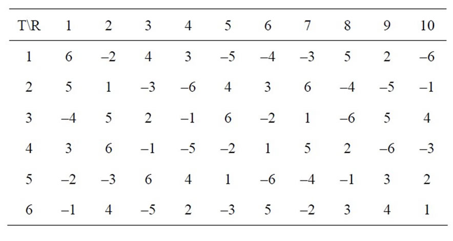
Table 1. Showing a sample double round-robin schedule for n = 6 with table representation.
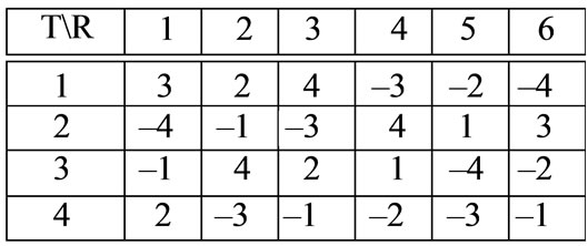
every TTP instance satisfying double round-robin constraint with n teams can be converted to an instance of the graph coloring problem with n × (n – 1) vertices, with each vertex being of degree 4n – 7 and 2n – 2 colors. Consequently, each possible coloring scheme for the specified graph corresponds to a unique schedule for the TTP instance. This particular representation is applied in a subroutine in the proposed SA algorithm in order to obtain neighbors for the local search procedure. Figure 1 depicts two equivalent representation of a schedule for a TTP instance with 4 teams; one by the discussed table representation, the other one by graph coloring scheme.
As a result, TTP instances can be viewed as graph coloring problem instances with a slight difference. Instead of merely searching for a coloring scheme (i.e. any assignment of labels to vertices such that no adjacent vertices have the same label), a particular one is sought which minimizes an objective function; thus, converting the graph coloring problem to an optimization problem.
4. Local Search in SA Algorithm for the TTP
This paper proposes a Simulated Annealing (SA) algorithm for the TTP. SA is an efficient local search algorithm that can be applied effectively to solve numerous combinatorial optimization problems. The algorithm
 (a)
(a) (b)
(b)
Figure 1. Two equivalent schedules for a TTP instance with n = 4, represented by a graph coloring scheme (a), and a table representation (b). The ordered pairs inside the nodes of the graph are individual games and the labels appearing beside them are the round, in number, which they are scheduled in.
starts with an initial configuration (i.e. a double roundrobin schedule). Its basic steps move from a current configuration c, to a configuration in the neighborhood of c. The SA algorithm follows certain properties such as:
1) It explores both feasible and infeasible solutions. The constraints are divided into two categories: hard constraints which are always satisfied and soft constraints which may or may not be violated. The hard constraints are round-robin constraints, while the soft constraints are no-repeat and at-most constraints. In other words, all schedules in the search space are round-robin schedules which may or may not satisfy the no-repeat or at most constraint. Exploring infeasible solutions as well as feasible ones seems to be crucial to the performance of the algorithm; since, a good solution may be reached through an infeasible one.
2) It dynamically modifies the objective function which is elaborated in this section, to balance the time spent in feasible and infeasible regions.
3) As the temperature descends in SA procedure, it becomes more likely for the search to be entrapped in local minima. Thus the SA algorithm uses reheats (e.g. [18]) to evade such situations.
4.1. The Neighborhood Structure in SA Algorithm
The neighborhood of a schedule is defined as the set of schedules which can be obtained by applying the following moves to it. The goal is to create similar schedules, whether feasible or not, to the current schedule with minimal alterations in order to provide a well distributed and continuous search space to the problem. The first five moves are the same as the moves suggested by Anagnostopoulos et al. [3] and the last one is called Kempe move proposed in [19].
• SwapHomes(S, Ti, Tj). This move swaps the order in which team Ti plays against team Tj at its home or away. In others words, if according to S, it is scheduled for team Ti to play against team Tj at rounds rk and rl at home and away respectively, SwapHomes(S, Ti, Tj) is the same schedule as S except that now the two games between teams Ti and is Tj held at Ti’s home at round rl and at Tj’s home at round rk
• SwapRounds(S, rk, rl). The move simply swaps rounds rk and rl [3].
• SwapTeams(S, Ti, Tj). This move swaps the schedules of teams Ti and Tj, except for the games that they play against each other.
• PartialSwapRounds(S, Ti, rk, rl). This move considers team Ti and swaps its games at rounds rk and rl. Then the rest of the schedule for rounds rk and rl is updated (in a deterministic way) to produce a double roundrobin tournament.
• PartialSwapTeams (S, Ti, Tj, rk). This move considers round rk and swaps the games of teams Ti and Tj. Then, the rest of the schedule for teams Ti and Tj (and their opponents) is updated to produce a double round-robin tournament.
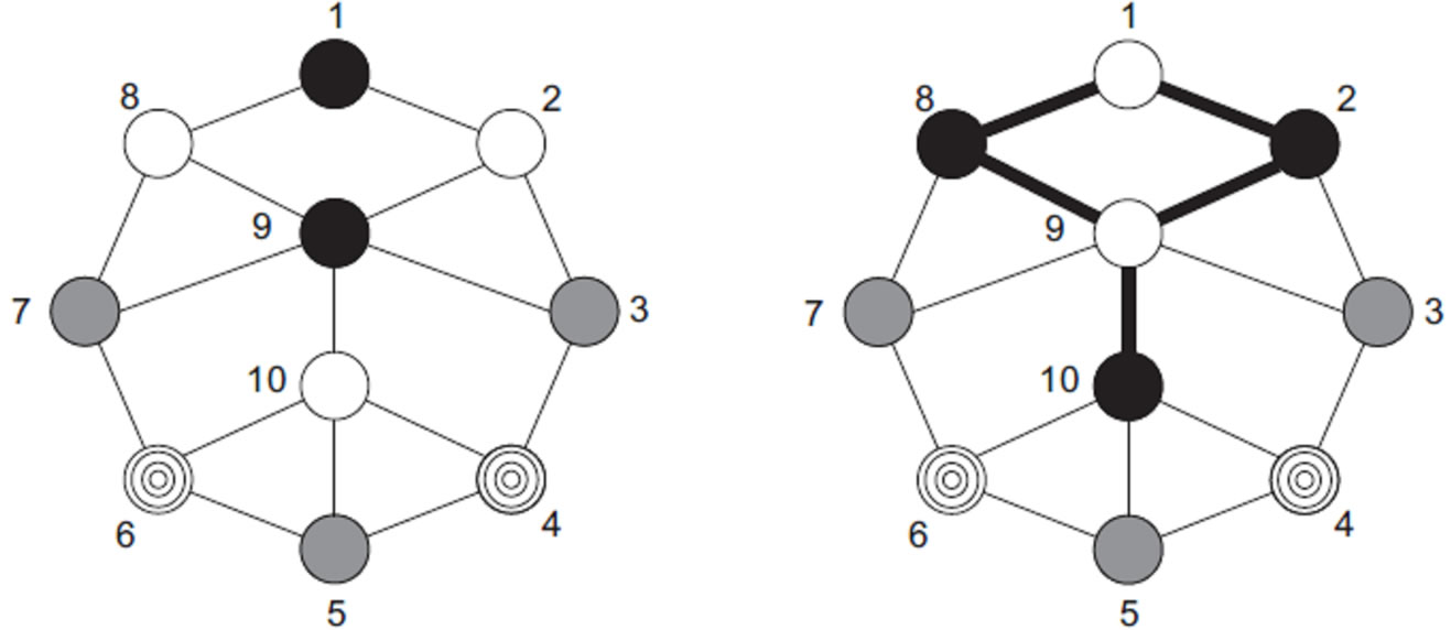
Following the correspondence between graph coloring problems, a promising strategy for exploring the space of solutions is presented by [19], applying the Kempe-chain operators. A Kempe-chain neighborhood takes a graph G and involves identifying a connected sub-graph that contains exactly 2 colors. If G is feasibly colored (i.e. it contains no pairs of adjacent vertices with the same color), then swapping the colors of all vertices within such a sub-graph will lead to a new feasible coloring that uses no more colors than the original. A demonstration of this process is given in Figure 2 where we use the notation Kempe(v, c) to denote a move that involves a particular selected vertex v and color c (where v is not currently assigned to color c).
• KempeChainMove(S, Ti, rk, rl). This move applies Kempe(v, c) move to the graph G = (V, E) corresponding to the TTP with coloring C corresponding to schedule S to obtain a new schedule if possible; where vertex  represents the game that team Ti is scheduled to play at round rk against its opponent, say team Tj, and rl is of course any round other than rk. In other words, it moves the game between teams Ti and Tj from round rk to rl.
Smart Moves
The algorithm has two key properties which we call in advancing in the search space. It is empirically observable that these properties have great positive influence on the performance of the algorithm.
1) The moves are not uniformly selected. Each move has a different disparate probability to be chosen by the algorithm to obtain a new schedule. More complex moves, namely KempeChainMove and PartialSwapTeams which obtain schedules with more nontrivial modifications are more likely to be applied in each step. This way the algorithm explores a greater portion of the search space in less time. Figure 3 depicts Kempe move being carried out on a sample coloring for a particular graph.
2) The parameters taken by each move as inputs are selected randomly but not uniformly. For each specific move, if applying a particular combination of parameters to an infeasible schedule decreases the number of violations, is more likely to be chosen. For instance, assume that SwapRounds is chosen to obtain a neighbor. Two rounds should be passed to this move as input parameters. The probability distribution over all rounds is not uniform. Meaning that every round has the probability to be chosen and this probability is a function of its violations in at-most and/or no-repeat constraint, i.e. the more

Figure 2. The effects of Kempe move probability on the final found solutions (NL10).
 (a) (b)
Figure 3. Demonstrating the function of Kempe move. (a) A graph being colored by four distinct colors, say the color of vertex 1 is white and the color of vertex 2 is black. (b) The same graph after applying Kempe (1, black) to it which has yielded another consistent coloring for the graph.
violation one round causes the more probability it has to be chosen.
It is observed that these heuristic strategies in choosing a neighbor have significant impact on the outcome of the algorithm. Better adjusted probabilities lead to higher quality schedules in less time.
4.2. Initial Solutions
The algorithm exploits a greedy scheme in order to generate an initial random schedule satisfying the hard constraints. This greedy scheme is discussed in [19]. It starts with sorting the games in lexicographic order, if they are represented in ordered pairs like {i, j}. For instance, for n = 10 the matches are ordered as {0, 1}, {0, 2}, {0, 3}, ···, {8, 9}. Then the first match is assigned to the first round and afterwards each remaining match is considered in turn and assigned to the next round where no Interference occurs. This way a single round-robin schedule (SRR) is obtained and a double round-robin schedule is constructed by replicating the SRR schedule in the remaining rounds and then swapping all of {i, j} ordered pairs in the replicated section to {j, i}. This greedy scheme in computational experiments takes less than a second to be performed for instances with large n. Following this procedure, the graph coloring representation of the schedule will be created by simply labeling each individual game (vertex of the graph corresponding to the TTP instance) with the round it is scheduled in. Afterwards, the Kempe neighborhood move is applied to this schedule about a hundred times in order to obtain another one. This final schedule can be considered approximately random in the search space. In other words, appearance of any schedule satisfying hard constraints can be considered roughly equal. These two steps take imperceptible time to be performed and it is as an efficient way to obtain a random initial solution for the SA algorithm.
4.3. Simulated Annealing for TTP
As mentioned before, the algorithm uses a simulated annealing meta-heuristics to explore the search space (i.e. the neighborhood graph). It starts by a random schedule which is obtained by a greedy algorithm explained in the previous section. Then, it follows the conventional simulated annealing algorithm schema. Given a temperature T, the algorithm randomly selects one of the schedules in the neighborhood of the current schedule yielded by the specified moves, and computes the difference Δ in the objective function produced by the move. If Δ < 0, the algorithm applies the move. Otherwise it applies the move with probability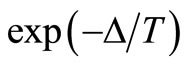 . As it is intentioned in simulated annealing, the probability of accepting a non-improving move decreases over time. This behavior is obtained by decreasing the temperature as follows. A variable counter is used which is incremented for each non-improving move and reset to zero when the best solution found so far is improved. When counter reaches a particular upper limit, the temperature is updated to
  (where β is a fixed constant smaller than 1) and counter is reset to zero.
4.4. The Objective Function
As discussed before, the schedules in the SA algorithm may or may not satisfy certain constraints, namely at-most and no-repeat. Furthermore, it is not guaranteed that the moves maintain the feasibility even if the search is initiated with a feasible schedule. It is crucial to the performance of the algorithm that the search goes through the infeasible schedules as well as the feasible ones, as it is likely that a solution can be reached through a series of infeasible schedules. Consequently, the standard objective function, as stated in [3], is altered so as to yield another objective function which makes use of the number of violation besides travel distance, therefore exploring the infeasible space as well.
The new objective function is defined as follows:
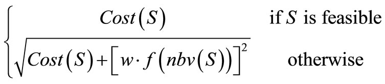
where the nbv(S) denotes the number of violations of the no-repeat and at-most constraints, w is a weight, and f: n → n is a sub-linear function such that f(1) = 1. Anagnopostopoulus et al. [3] suggests that
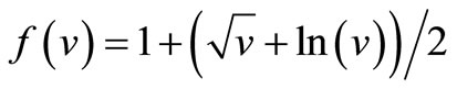
is a suitable function to control the violations of the TTP’s solutions.
5. Computational Experiments
The proposed SA algorithm is tested on a number of instances of the TTP with no-repeat and at-most constraints. The instances, i.e. the NLn instances are based on the information in Major League Baseball. The optimal solution for NL4, NL6 and NL8 has been reported in the literature, e.g., see [6]. The algorithm proposed by this paper as well leads to optimal solution for these instances, significantly improving the time performance and the quality of the best found solution for other instances. More specifically, the computational time of this algorithm, compared to that of other studies is considerably decreased for NL6 through NL10. Table 2 demonstrates the comparison of the results of the proposed algorithm with that of earlier researches, namely Simulated Annealing, LR-CP, a hybrid Simulated Annealing-Hill Climbing approaches and a hybrid PSO-SA approach which are respectively proposed in [3,20,21] and [22]. The detail of these methods can be found in [17].
For each NLn, the algorithm was run several times; accordingly the Best Found Solution (BFS) and Total Running Time (TRT) of the execution of the procedure is reported for each n. These experiments were performed on an Intel® Core™i5 CPU with 2.40 GHz clock rate and a main memory of 2 GB. Also, the program implementing the algorithm was written in C++ programming language and MinGW GCC was used to compile the
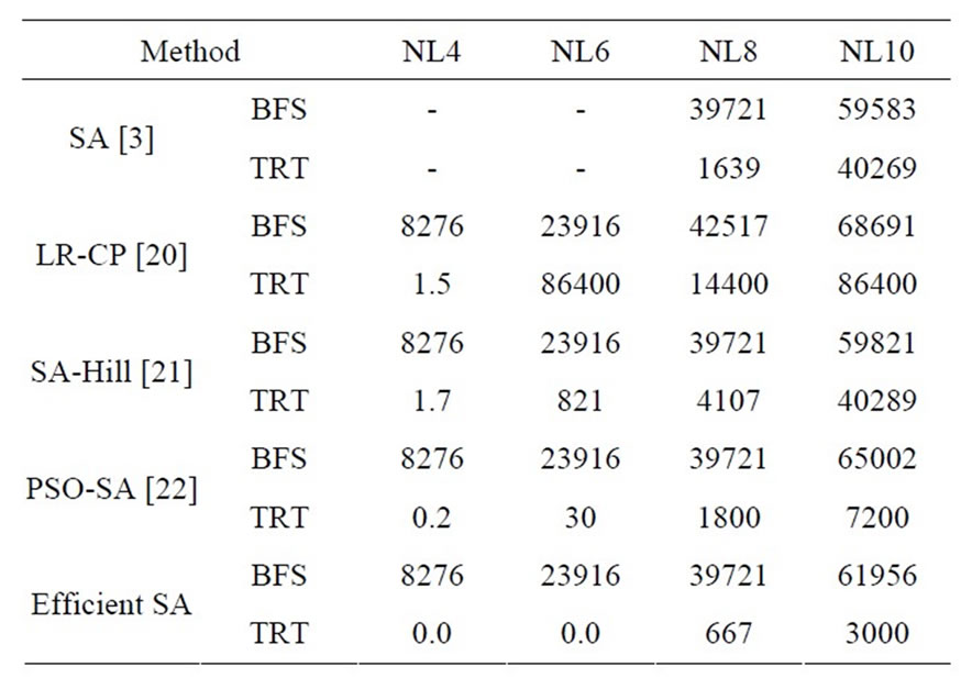
Table 2. Results and comparison of the performances of proposed solution methods for the traveling tournament problem.
program.
The parameters of the SA algorithm in the running which are reported are set to the values that appear in Table 3. Refer to [3] for detailed description for each of these parameters. These parameters have been found suitable corresponding to different problem sizes. It can be observed that with the size of the problem increasing, it is better for the SA algorithm to start with higher initial temperatures (T0). This prevents the algorithm to get stuck in local minima early in the process of the search, when n becomes greater. However, unlike the parameters in [1], these initial temperatures are not increasing linearly with respect to n.
Figure 4 indicates the importance of the parameter β. In this figure our solutions obtained for NL10 by the algorithm by applying different β values. For each β, the corresponding instance is solved several times and the best one is selected. Note that these runs continued for 3000 seconds the best solution is obtained for β = 0.99 which is the least value.
Finally, Figure 2 demonstrates the influence of Kempe move on improving the solutions found by the SA algorithm. As it was mentioned before, each neighborhood movement has different probability in order to explore the search space more thoroughly and efficiently. For each Kempe move probability, the instance corresponding to NL10 is solved several times and the best final solution is determined for each of these probabilities. Similar to the previous part, each run continued for 3000 seconds. It can be observed that by applying Kempe move more frequently to a particular point, approximately 0.5, better solutions can be obtained. However, further use of this move affects the algorithm negatively. Also, it can be inferred that the optimal values for the probability of Kempe move lies in the interval (0.4, 0.6).
6. Conclusion
Scheduling sports competitions has drawn significant attention to itself in recent years. This is a consequence of the involvement of considerable revenue for sports club, television networks as well as the involvement of dicult combinatorial optimization problems. This paper studies the Traveling Tournament Problem, a sports scheduling problem (TTP) which has been proposed in [1] and has originated from the scheduling of Major League Baseball of the United States and it models specific features of this sports event. Several recent researches regarding this problem have developed heuristic approaches to solve the problem. However, these works apply just one unique modeling to abstract the problem
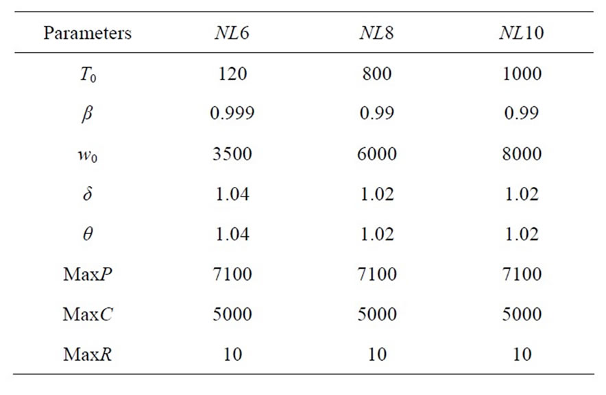
Table 3. Parameter values for computational experiments.
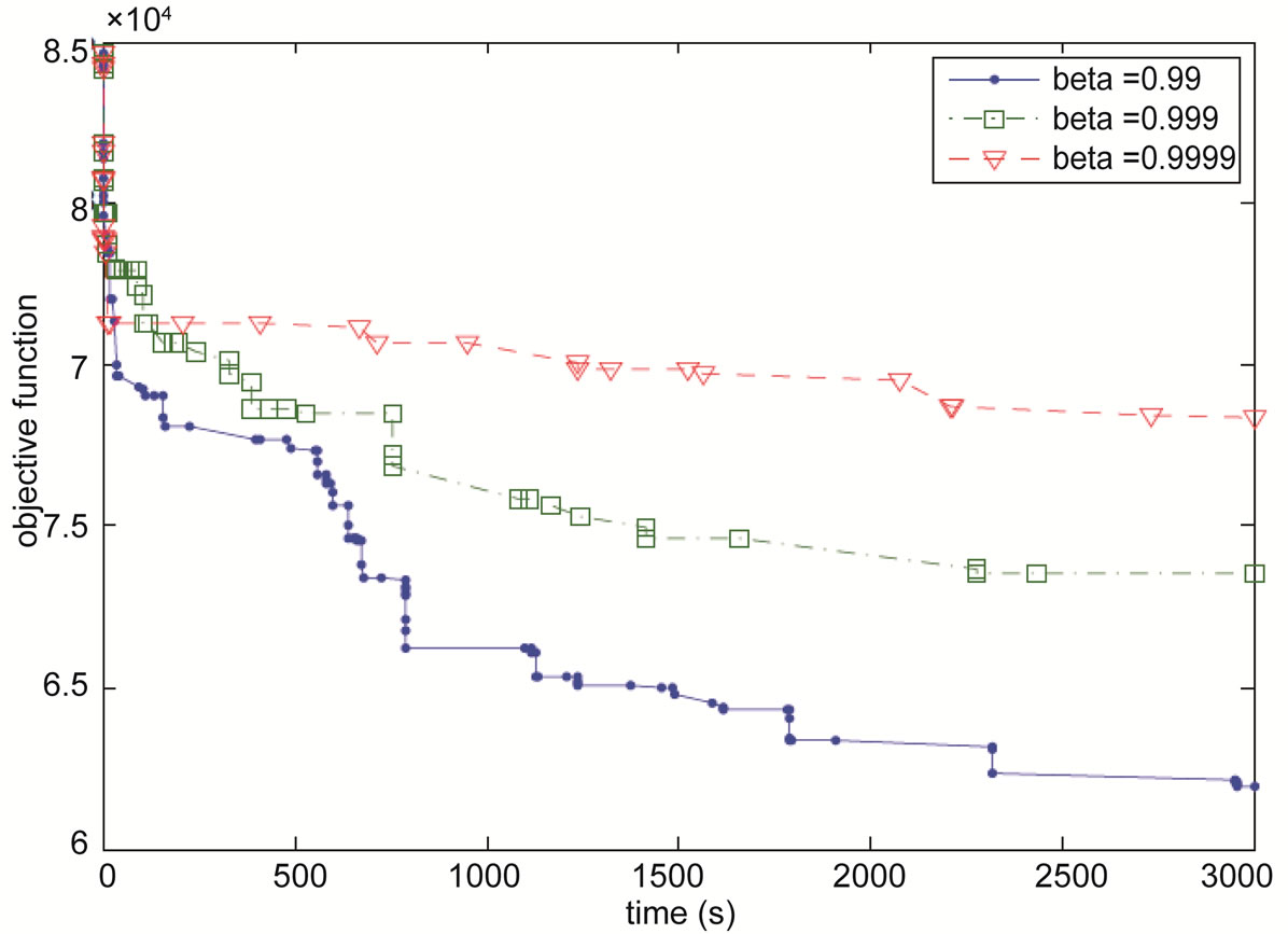
Figure 4. The effects of β on the solutions found by the SA algorithm over time (NL10).
features. For instance, either just tables model or an Integer Programming mathematical model [22]. Our paper applies graph coloring and table model simultaneously to exploit the properties of graph coloring problems as well in order to develop an efficient heuristic model based upon the algorithm proposed in [3]. This leads to a schedule modification technique, that is Kempe move, discussed in [19] which we use in combination with a greedy scheme to generate a high quality initial solution to the SA algorithm. Additionally, this graph theoretical technique is used to better explore the space of solutions. Also, the neighborhood in SA algorithm is explored more effectively by using the techniques called smart moves. The experimental results indicate that this particular technique improves the efficiency of the algorithm, indeed.
This paper has not considered a hybrid method in order to improve the solutions. There is the possibility of applying a Genetic Algorithm (GA) on the schedules explored by the SA algorithm. This process can be done sequentially with the simulated annealing algorithm. Moreover, new methods for exploring neighborhoods in the search space can contribute to the performance of the SA algorithm.
REFERENCES
- A. K. Easton, G. Nemhauser and M. Trick, “The Traveling Tournament Problem: Description and Benchmarks,” Lecture Notes in Computer Science, Vol. 2239, 2001, pp. 580-585. doi:10.1007/3-540-45578-7_43
- J. C. Bean and J. R. Birge, “Reducing Travelling Costs and Player Fatigue in the National Basketball Association,” Interfaces, Vol. 10, No. 3, 1980, pp. 98-102. doi:10.1287/inte.10.3.98
- A. Anagnostopoulos, L. Michel, P. Van Hentenryck and Y. Vergados, “A Simulated Annealing Approach to the Traveling Tournament Problem,” International Workshop on Integration of AI and OR Techniques, Montreal, 2003.
- J. A. M. Schreuder, “Constructing Timetables for Sport Competitions,” Mathematical Programming Study, Vol. 13, 1980, pp. 58-67. doi:10.1007/BFb0120907
- D. de Werra, “Scheduling in Sports,” Studies on Graphs and Discrete Programming, 1981, pp. 381-395.
- D. de Werra, “Some Models of Graphs for Scheduling Sports Competitions,” Discrete Applied Mathematics, Vol. 21, No. 1, 1988, pp. 47-65. doi:10.1016/0166-218X(88)90033-9
- R. T. Campbell and D. S. Chen, “A Minimum Distance Basketball Scheduling Problem,” Management Science in Sports, Studies in the Management Sciences, Vol. 4, 1976, pp. 15-26.
- D. Costa, “An Evolutionary Tabu Search Algorithm and the NHL Scheduling Problem,” Information Systems and Operational Research, Vol. 33, 1995, pp. 161-178.
- M. B. Wright, “Scheduling Fixtures for Basketball New Zealand,” Computers & Operations Research, Vol. 33, No. 7, 2006, pp. 1875-1893. doi:10.1016/j.cor.2004.09.024
- T. Benoist, F. Laburthe and B. Rottembourg, “Lagrange Relaxation and Constraint Programming Collaborative Schemes for Traveling Tournament Problems,” International Workshop on Integration of AI and OR Techniques, Ashford, Kent, 2001.
- K. Easton, G. Nemhauser and M. Trick, “Solving the Traveling Tournament Problem: A Combined Integer Programming and Constraint Programming Approach,” Lecture Notes in Computer Science, Vol. 2740, 2003, pp. 100-109. doi:10.1007/978-3-540-45157-0_6
- J. H. Lee, Y. H. Lee and Y. H. Lee, “Mathematical Modeling and Tabu Search Heuristic for the Traveling Tournament Problem,” Lecture Notes in Computer Science, Vol. 3982, 2006, pp. 875-884. doi:10.1007/11751595_92
- K. K. H. Cheung, “Solving Mirrored Traveling Tournament Problem Benchmark Instances with Eight Teams,” Discrete Optimization, Vol. 5, No. 1, 2008, pp. 138-143. doi:10.1016/j.disopt.2007.11.003
- N. Fujiwara, S. Imahori, T. Matsui and R. Miyashiro, “Constructive Algorithms for the Constant Distance Traveling Tournament Problem,” The International Series of Conferences on the Practice and Theory of Automated Timetabling, 2006, pp. 402-405.
- L. D. Gaspero and A. Schaerf, “A Composite-Neighborhood Tabu Search Approach to the Traveling Tournament Problem,” Heuristics, Vol. 13, No. 2, 2007, pp. 189-207. doi:10.1007/s10732-006-9007-x
- S. Urrutia and C. C. Ribeiro, “Maximizing Breaks and Bounding Solutions to the Mirrored Traveling Tournament Problem,” Discrete Applied Mathematics, Vol. 154, No. 13, 2006, pp. 1932-1938. doi:10.1016/j.dam.2006.03.030
- M. A. Trick, “Michael Trick’s Guide to Sports Scheduling”. http://mat.gsia.cmu.edu/TOURN/
- D. T. Connelly, “General Purpose Simulated Annealing,” Journal of Operations Research, Vol. 43, 1992, pp. 495- 505.
- R. Lewis and J. Thompson, “On the Application of Graph Coloring Techniques in Round-Robin Sports Scheduling,” Computers and Operations Research, Vol. 38, No. 1, 2011, pp. 190-204. doi:10.1016/j.cor.2010.04.012
- J. Kennedy and R. C. Eberhart, “A Discrete Binary Version of the Particle Swarm Algorithm,” 1997 IEEE International Conference on Computational Cybernetics and Simulation, Piscatawary, Orlando, 12-15 October 1997, pp. 4104-4109.
- A. Lim, B. Rodrigues and X. Zhang, “A Simulated Annealing and Hill-Climbing Algorithm for the Traveling Tournament Problem,” European Journal of Operational Research, Vol. 174, 2006, pp. 1459-1478. doi:10.1016/j.ejor.2005.02.065
- M. B. Wright, “Scheduling Fixtures for Basketball New Zealand,” Computers & Operations Research, Vol. 33, No. 7, 2006, pp. 1875-1893. doi:10.1016/j.cor.2004.09.024