American Journal of Operations Research
Vol. 2 No. 1 (2012) , Article ID: 17839 , 11 pages DOI:10.4236/ajor.2012.21015
A New Approach for Ranking Efficient Units in Data Envelopment Analysis and Application to a Sample of Vietnamese Agricultural Bank Branches
1Water Resources University, Hanoi, Vietnam
2Military Technical Academy, Hanoi, Vietnam
3Air Defence-Air Force Academy, Hanoi, Vietnam
Email: khacminh@gmail.com, van_khanh1178@yahoo.com, tuan.p83@gmail.com
Received February 1, 2012; revised March 5, 2012; accepted March 13, 2012
Keywords: Data Envelopment Analysis (DEA); Slacks-Based Measure of Efficiency (SBM); SCI Super-Efficient
ABSTRACT
This paper proposes a new approach for ranking efficiency units in data envelopment analysis as a modification of the super-efficiency models developed by Tone [1]. The new approach based on slacks-based measure of efficiency (SBM) for dealing with objective function used to classify all of the decision-making units allows the ranking of all inefficient DMUs and overcomes the disadvantages of infeasibility. This method also is applied to rank super-efficient scores for the sample of 145 agricultural bank branches in Viet Nam during 2007-2010. We then compare the estimated results from the new SCI model and the exsisting SBM model by using some statistical tests.
1. Introduction
DEA is a non-parametric approach of frontier estimation, first developed by Charnes, Cooper, and Rhodes (CCR) [2]. Based on the original CCR model, Banker, Charnes, and Cooper (BBC) [3] developed a variable returns to scale (VRS) variation. Various researchers have developed DEA ever since. A large number of empirical studies have adapted these models to deal with real economic problems. One adaptation is to rank decision-making units (DMUs), such as firms or industries. DMUs are divided into efficient and inefficient groups, and their ranks can be examined by using DEA.
According to Adler et al. [4], the research on ranking DMUs could be classified into six streams, including 1) cross-efficiency ranking methods; 2) benchmark ranking method; 3) ranking with multivariate statistics in the DEA context; 4) ranking inefficient DMUs; 5) DEA and multi-criteria decision-making methods; and 6) superefficiency ranking techniques. The sixth stream is superefficiency ranking techniques developed by Andersen and Petersen [5], which ranked efficiency units by measuring the distance from an efficiency unit to a frontier, based on a set of observations excluding the efficiency unit in question. In other words, the most efficient unit is the one that can proportionally reduce outputs relative to the most efficient one without becoming inefficient. The approach has become very popular and a lot of research work has extended this idea. Liu and Tsai [6] introduced tools for reconciling diverse measures, which characterize the profitability of the twenty-nine public semiconductor companies in Taiwan. To analyze their profitability performance, the companies used five variables, including three inputs and two outputs. Their procedure included five phases. In phase I, the companies used the super-SBM model to distinguish the efficient and inefficient companies. In phase II, the companies used the super-SBM model to obtain the projection points of the efficient companies on the frontier. These projection points constructed the secondary frontier. In phase III, they located the projection of inefficient companies on the secondary frontier. In phase IV, they used a linear programming technique to determine the set of weights of the indices for all the points on the secondary efficient frontier. Lastly, in phase V, they traced back the efficiency score of each company by multiplying the absolute efficiency score of its projection point on the secondary score obtained from the phase II and phase III. Lotfi et al. [7] presented the idea of computing the efficiency of DMUs with interval data. An interval was defined for the efficiency score of each unit. Lotfi et al. [7] examined a method for ranking DMUs by obtained efficiency interval. Their method was applied to commercial bank branches in Iran. Recently, Li et al. [8] developed a super-efficiency model to overcome some deficiencies in other models. They showed that their model was superior to that of both Andersen and Petersen [5] and Mehrabian et al. [9] by removing deficiencies in these models. Li et al. [8] also compared their model with slacks-based model developed by Tone [10], who presented a new super-efficiency model based on the work of Andersen [5]. However, Tone’s [9] super-efficiency model could not be applied to rank inefficient DMUs. In the section 2, we present the new approach, the section 3 applies the new approach to bank branches, including previous studies on banking performance, bank input and output, super-efficiency scores from SCI model, and the comparison of SBM and SCI models. The last section provides concluding remarks.
2. Theoretical Model
We analyze DMUs with the input and output matrices  and
and . It is assumed that the data set is positive, i.e.
 , and
, and . In order to estimate the efficiency of a
 , we formulate the following fractional program in the following equation:
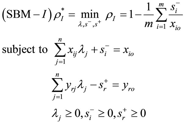 (1)
(1)
Definition 1. A  is SBM-I efficient only if
  and
and .
.
The CCR model can be formulated as the following:
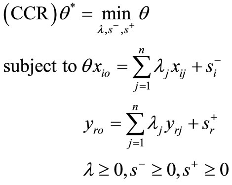 (2)
(2)
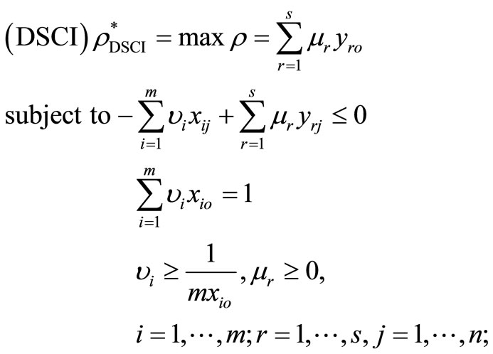
From the SBM-I model and the CCR model, we consider the following model:
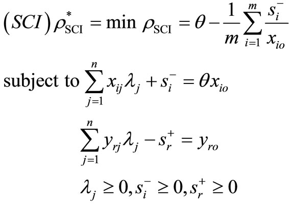 (3)
(3)
Definition 2. A  is SCI efficient only if
  and
and .
.
Theorem 1.  is SBM-I-efficient only if it is SCI-efficient.
Theorem 2.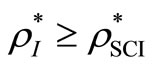 .
.
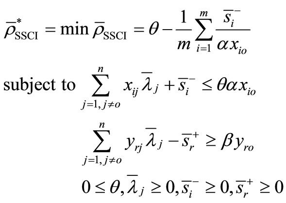
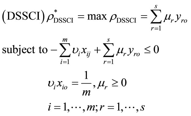
For , we have the following super-efficiency model:
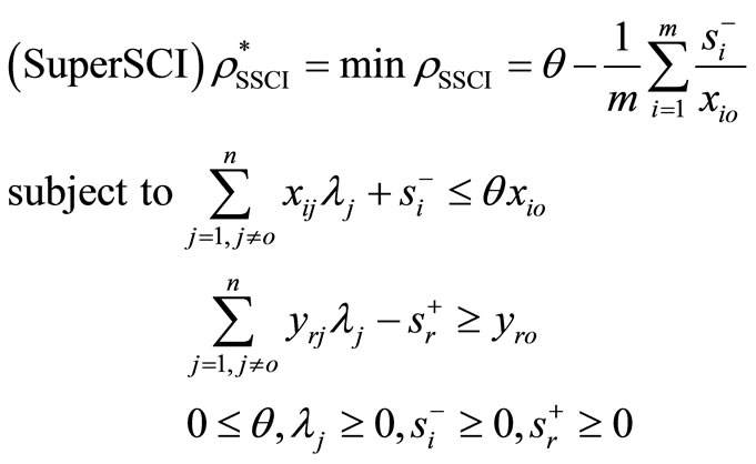 (4)
(4)
Theorem 3. The SCI super-efficiency model is always feasible under constant or variable return to scale assumption.
Proof. For any non-negative set 
we can define:
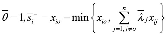
for all  and
and
for all  then
then
and
It is observed that
is a feasible solution to the model (4). Therefore, the model (4) is always feasible. This remains true under the assumption of VRS where  is added into the model (4).
Theorem 4. Let  with
with  and
and  be a DMU with reduced inputs and enlarged outputs compared with
 . Then, the SCI super-efficiency score of
  is not less than that of
 .
.
Proof. The optimal value to the model (4) for  is obtained by solving the following problem:
 (5)
(5)
Provide an optimal solution:
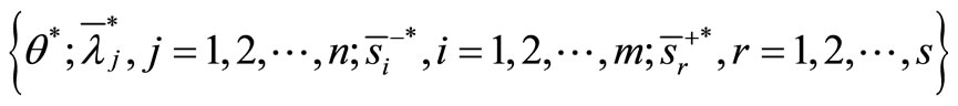
Then,
It is observed that
is a feasible solution to the model (4). Furthermore,
Theorem 5: For SCI model and the SCI super-efficiency model considering any DMUs, there are three possible cases:
• Case 1: The SCI super-efficiency optimal value of 
 , then
  is SCI model of inefficient decision making unit.
• Case 2: The SCI super-efficiency optimal value of 
 , then
  is SCI model of inefficient decision making unit or
  (
( is the set of efficient but not extremely efficient decision making units, F is the set of weak-efficient with non-zero slacks decision making units).
• Case 3: The SCI super-efficiency optimal value of 
 , then
  (E is the set of extremely efficient decision-making units).
Proof. The dual program of the problem in (3) and in (4) can be expressed as the following with the dual variables 
 (6)
(6)
 (7)
(7)
• Case 1: If the SCI super-efficiency optimal value of 
 , then
  and
and  , which indicates that
  is a optimal solution of model (6). Furthermore,
  is SCI model of inefficient decisionmaking unit.
• Case 2: If the SCI super-efficiency optimal value of 
 , from the proof of case 1, we have if
  is a feasible solution of model (7) and
  then
then  is also a feasible solution of model (6).
Assumption  is an optimal solution of model (4), then
If  is extremely efficient for model (3), then it has unique optimal solution
 ,
,  ,
, . So the above inequality cannot be satisfied. Furthermore,
  is SCI model of inefficient decision making unit or
 .
.
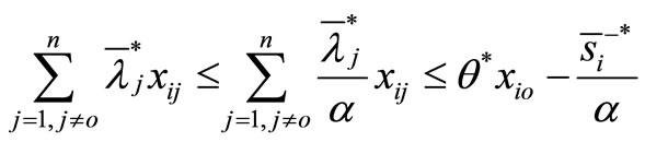
• Case 3: If  is a feasible solution of model (6), then,
It is shown that .
.
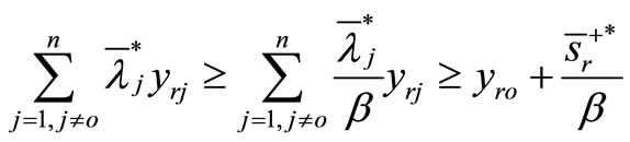
Furthermore,  is also a feasible solution of model (7) and
 . Suppose
  is extremely efficient for model (3), then by the above proof
  has a dual feasible multiplier; hence either (a)
  has an optimal multiplier
 , or (b) the multiplier program for
  in SCI super-efficiency is unbounded. If (b) holds, from theorem 2, we have
 , then
  is not extremely efficient, this is a contradiction. If (a) holds, from the proof of case 1 and case 2, we must have
 so
so .
.
3. Application to Vietnamese Agricultural Bank Branches
The structure of the agricultural bank has changed swiftly during the transition, in which the number of bank branches and the volume of capital transactions have increased over time. The agricultural bank has greatly contributed to the development of financial markets, especially the development of agricultural sector in Viet Nam. Studying production efficiency of the agricultural bank branches is thus necessary for promoting further contribution of the agricultural bank to the economy, as well as for proposing policy strategies for development of the agricultural sector under globalization. However, there have been a few quantitative studies that focus on measuring production efficiency of the commercial banks in Vietnam, and most of the current studies were based on qualitative analyses. Therefore, the objectives of this application are to estimate efficiency levels for the agricultural bank branches in Vietnam and to rank these bank branches according to their efficiency score in order to identify the most and the least efficient bank branches.
3.1. Previous Studies on Banking Performance
At the microeconomic level, efficiency is a concept to measure how efficiently the resources like inputs are used to produce an output of a defined final product. For the banking sector, the problem is rather complicated, because of the difficulties in defining the final products. For instance, should bank deposits be traced as an input or an output, and how should off-balance sheet items be treated? There are two main approaches for choosing input and output variables, including the value-added approach, and the asset approach or intermediation approach. The valued added approach is based on the share of value added to identified inputs and outputs for the banking sector. This approach considers deposits as outputs since they imply the creation of value added. The intermediation approach is based on the theory of intermediation, which considers banks as financial intermediation between depositors and borrowers. In this approach, liabilities are considered as inputs and assets as output. In fact, many studies have applied intermediation approach in DEA analysis. For instance, Favero and Papi [11] estimated the technical efficiency of 174 Italian banks in 1991 by using four inputs (labour, capital, loanable funds, and financial capital), and three outputs (loans, investments, and non-interest income). The estimated results were robust to modifications in the specification of inputs, and outputs followed the intermediation and asset approaches.
Wheelock and Wilson [12] used non-parametric approach to compute the Malmquist index and productivity change for all U.S. banks during 1984-1993. They used three inputs (labour, physical capital, and purchased funds) and five outputs (real estate loans, commercial and industrial loans, consumer loans, all other loans, and total deposits), and found that the average productivity growth of larger banks was 3.44% per year during 1984- 1990. Using data of 1490 banks of German banking, Lang and et al. [13] evaluated the banking technology by applying the intermediation approach, which treated deposits as inputs and loans as outputs.
Asmild et al. [14] used data envelopment analysis (DEA) window analysis to evaluate the industry’s performance overtime during 1981-2000. To measure productivity changes overtime, they used Malmquist indices, calculated from DEA scores. To define the “same period frontier” in a DEA window analysis, Asmild et al. [14] showed that for both the adjacent and the base period Malquist index and for all suggested definitions of same period frontier.
Camanho et al. [15] described an application of data envelopment analysis (DEA) to the performance assessment of Portuguese bank branches. They focussed on analyzing the relation between branch size and performance. Hauner et al. [16] considered bank efficiency and competition in low-income countries in the case of Uganda. The concern was that the state-dominated, inefficient, and fragile banking systems in many low-income countries, especially in sub-Saharan Africa, were a major hindrance to economic growth. They analyzed the impact of the far-reaching banking sector reforms undertaken in Uganda to improve competition and efficiency. They found that the level of competition has increased significantly and had been associated with a rise in efficiency. They showed that the larger banks and the foreign-owned banks had become more efficient, while smaller banks had become less efficient in the face of increased competitive pressures.
Wheelock et al. [17] considered new evidence on returns to scale and product mix among the U.S. commercial banks. They found that banks experience increasing returns to scale up to approximately $500 million of assets, and constant returns and minimum efficient scale had increased since 1985.
Chen [18] analyzed the technical efficiency of 39 banks in Taiwan using chance-constrained DEA and stochastic frontier analysis (SFA). He showed that there were significant differences in efficiency scores between chance-constrained DEA and stochastic frontier production function.
Nguyen et al. [19] estimated efficiency levels for 32 commercial banks in Vietnam during 2001-2005 and ranked these banks according to their efficiency scores in order to find the most and the least efficient banks. Efficiency was measured by data envelopment analysis (DEA) model and super-efficiency measure through SBM, in which the assumption of variable return to scale (VRS) was used. They conducted a sensitive analysis, in which data for the banks were allowed to simultaneously vary across different subsets of inputs and outputs.
3.2. Bank Input and Output
In this study, the selection of inputs and outputs for our model is based on the intermediation approach. The output categories include received interest (y1); other operating income (y2); and total loans (y3). The inputs include personnel expenses (x1); net total assets (x2), which are estimated by the total domestic assets minus bank loans and investments; all deposits (x3); and labour (x4). The study period is 2007-2010, in which the number of observations remains over time. Table 1 presents the statistical summary for the outputs and inputs of the sampled banks in the study period. Generally, the table shows that the Agricultural bank branches in Vietnam expanded over time in terms of all output and input indicators.
3.3. Data of Agricultural Bank Branches in 2007-2010
Data in our research, which was obtained from the Vietnamese Agricultural Bank, consist of annual observations of outputs and inputs from 145 agricultural bank branches during 2007-2010. Three outputs and four inputs are used in the empirical application of this study. The four inputs are personal expenses, net total assets, deposits and labour and three outputs are received interest, other interest income and loans. These input and output variables are defined in Table 1. Tables 2-5 present the statistical summary for the outputs and inputs of the sample banks in the study period. Generally, all tables show that the agricultural bank branches in Vietnam expanded over time in terms of output and input indicators. Note that, among the studied bank branches, there were 14 largest ones, which accounted for 33.5%, 31.5%, 30.6%, and 28.6% of the total assets of all 145 bank branches in 2007, 2008, 2009, and 2010, respectively. The 14 smallest bank branches in the sample only accounted for 1.2%, 2.5%, 2.7%, and 2.9% of total assets of the total sampled banks in the study period.
3.4. Super Efficiency Scores from SCI Model
The analysis produced sets of super-efficiency scores for each year from 2007 to 2010. They are the super-efficiency under the assumption of constant return to scale and the super-efficiency under the assumption of variable return to scale. The scores are presented as annual averages of bank branches under investigation for the whole Vietnamese Agricultural bank. Although average the super-efficiency scores causes loss of information, particularly the variation among individual bank branches would require a separate study. However ranking of each bank branches can capture information about bank branches’ super efficiency scores. Super-efficiency score is estimated using the Mathlab program with input-oriented model under the assumption of constant return to scale and variable return to scale for the sample of 145 Agricultural bank branches in Vietnam.
Table 6 presents the estimated results. Under the assumption of constant return to scale, the mean superefficiency of the sampled bank branches in 2007, 2008, 2009, and 2010 were 64%, 63%, 57%, and 59%, respectively. While, under the assumption of variable return to scale ,the mean super-efficiency of the sampled bank branches in 2007, 2008, 2009, and 2010 were 71%, 71%, 66%, and 67%, respectively. These results imply that on average, the sampled bank branches could produce the same output levels by using fewer resources than they employed in respective years.
As shown in Table 6, maximum and minimum superefficiency levels for the sampled bank branches under the assumption of constant return to scale (variable return to scale) varies from 1.328 (1.183), 1.434 (1.662), 1.56 (1.725), 1.481 (1.719) to 0.355 (0.374), 0.379 (0.401), 0.323 (0.359), 0.357 (0.380) in 2007, 2008, 2009, and 2010, respectively.
The frequency distribution of the mean super-efficiency scores estimated from SCI models under the CRS and VRS assumptions are presented in Tables 7-10. A
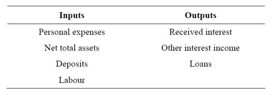
Table 1. Input and output variables.
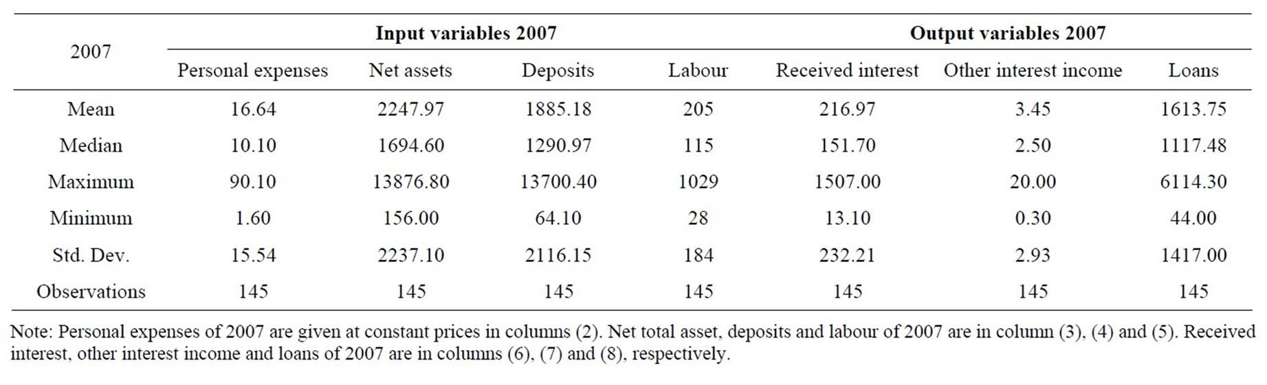
Table 2. Summary statistics—inputs and outputs in 2007.
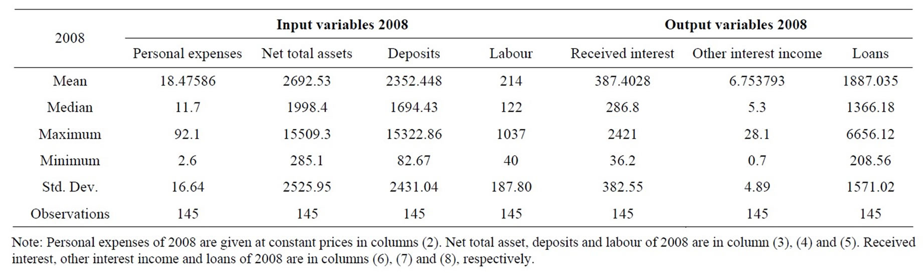
Table 3. Summary statistics—inputs and outputs in 2008.
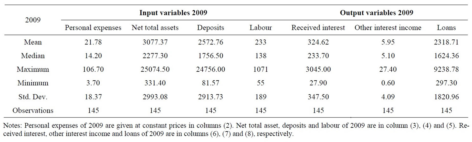
Table 4. Summary statistics—inputs and outputs in 2009.
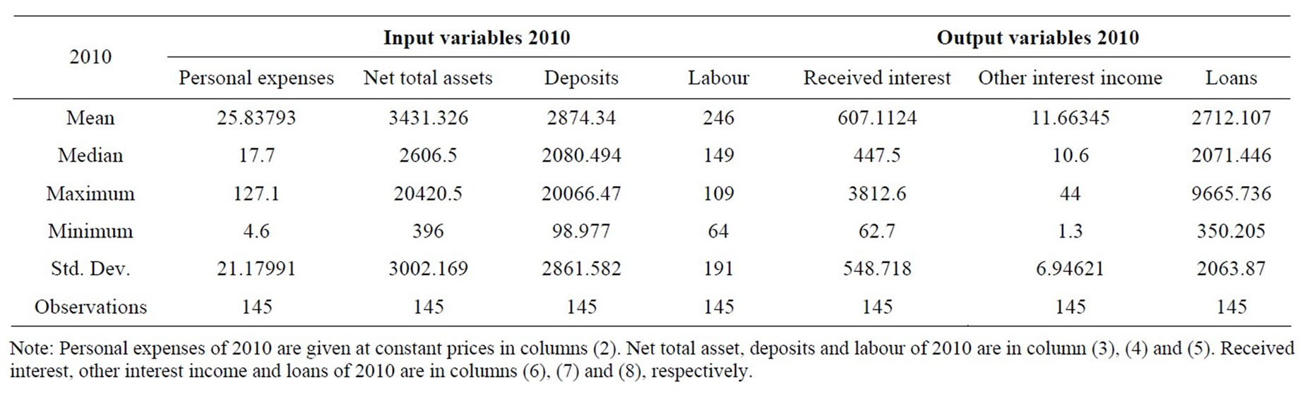
Table 5. Summary statistics—inputs and outputs in 2010.
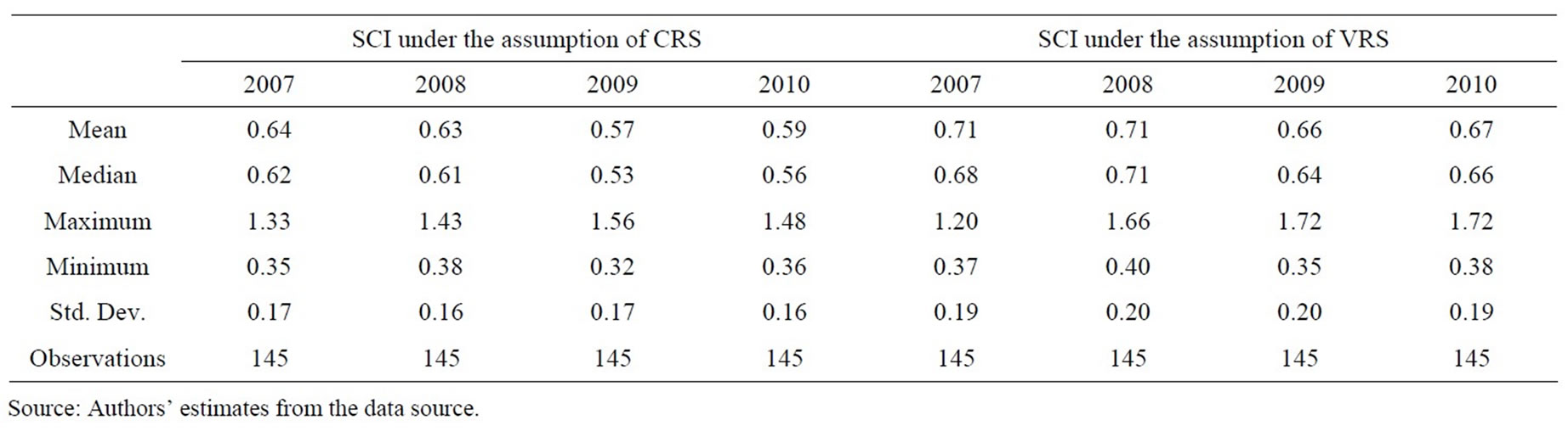
Table 6. General results of technical efficiency from SCI model.
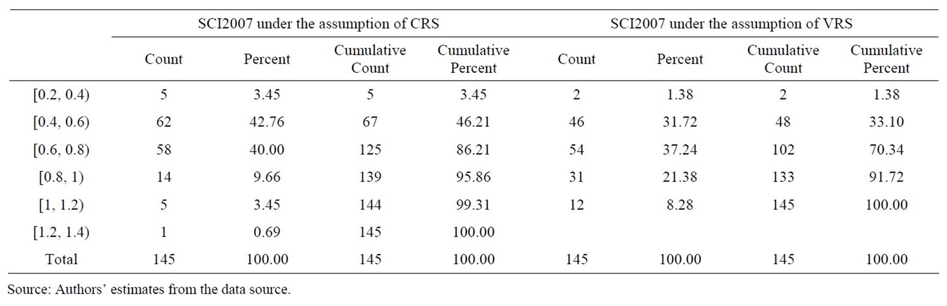
Table 7. Frequency distribution of super efficiency measures estimated under the assumptions of CRS and VRS from SCI model in 2007.
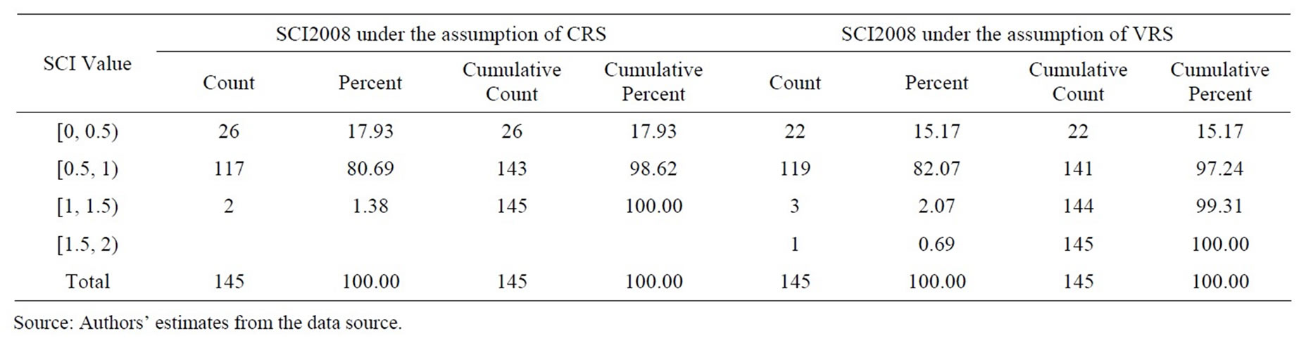
Table 8. Frequency distribution of super efficiency measures estimated under the assumptions of CRS and VRS from SCI model in 2008.
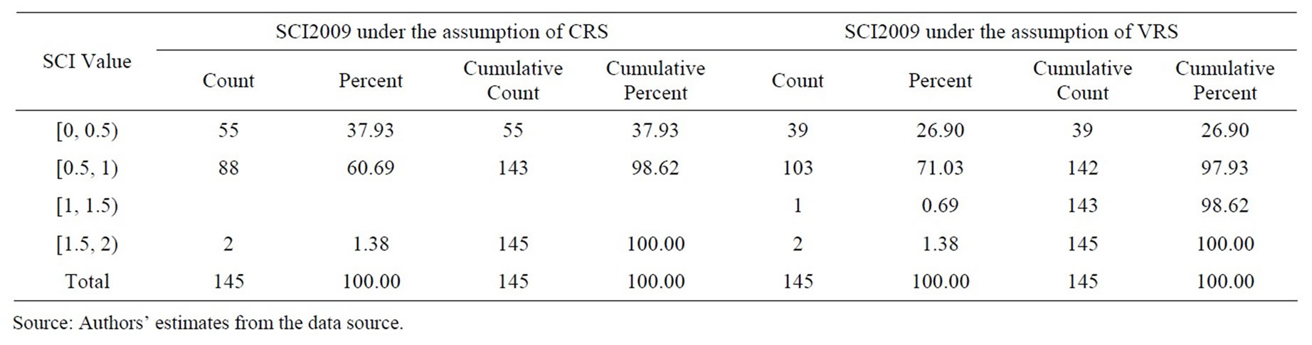
Table 9. Frequency distribution of super efficiency measures estimated under the assumptions of CRS and VRS from SCI model in 2009.
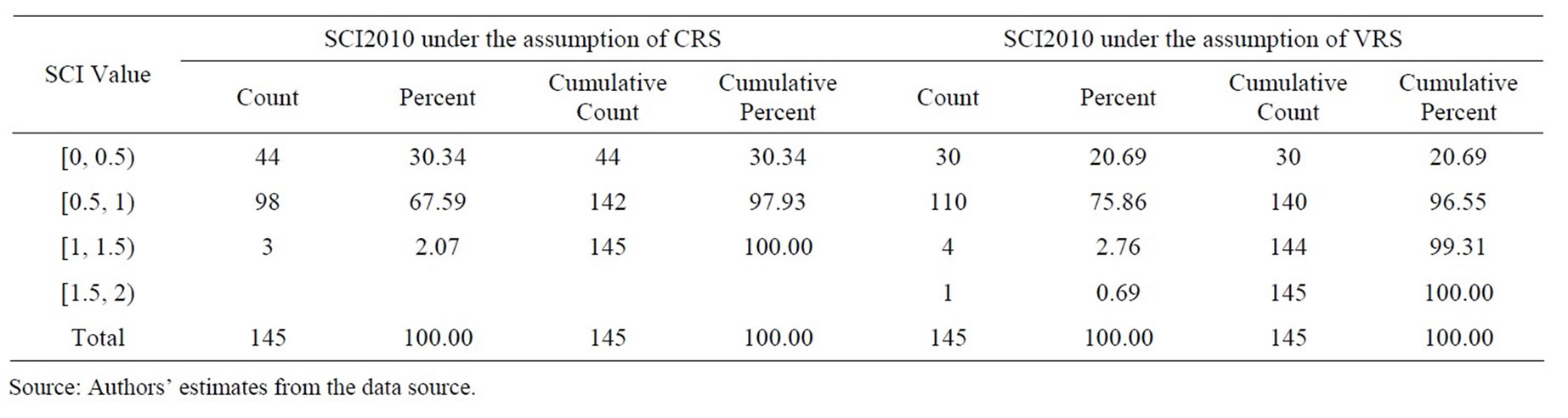
Table 10. Frequency distribution of super efficiency measures estimated under the assumptions of CRS and VRS from SCI model in 2010.
bank having efficiency of more than 100% was fully technically efficient. Therefore, in terms of super-efficiency, out of 145 bank branches in the sample, the number of fully technically efficient bank branches under the assumption of constant return to scale (variable return to scale) was 6 (12), 2 (4), 2 (3), and 3 (5) in 2007, 2008, 2009, and 2010, respectively. The number of bank branches with super-efficiency range of 50%—more than 100% under the assumption of constant return to scale (variable return to scale) was 119 (123), 100 (106), and 101 (115) in 2008, 2009, and 2010, respectively. As an exception, the bank with technical efficiency level lied in the range 0% - 20% under the assumption of constant return to scale (variable return to scale) was 5 (2).
3.5. Relation between Banks’ Total Assets and Super-Efficiency Scores
In this section, our analysis focuses on the relation between bank size (the total assets by proxy) and superefficiency scores. The question is whether in the study period the larger bank branches had higher super-efficiency score than did the smaller bank branches. To do so, we use Spearman rank correlation for testing the null hypothesis H0 (total assets and super-efficiency scores are independent). Results of the statistical tests of the null hypothesis are shown in Table 11. The Spearman rank correlation coefficients between total assets and super-efficiency scores estimated from SCI’s model (2007, 2008, 2009, and 2010) are positive, but not high. They show that we cannot reject the null hypothesis. It generally means that, the large bank might not have high super-efficiency score. In practice, for instance, the total assets of Hanoi bank branch was about five times higher than the total assets of the Quan 10 bank branch, but Quan10 bank branch was more efficient than Hanoi Bank branch; even Quan 10 was one of the top ranking bank branch under the assumption of CRS.
3.6. A Comparison of SBM and SCI Models
In this section, we compare the estimated results from the
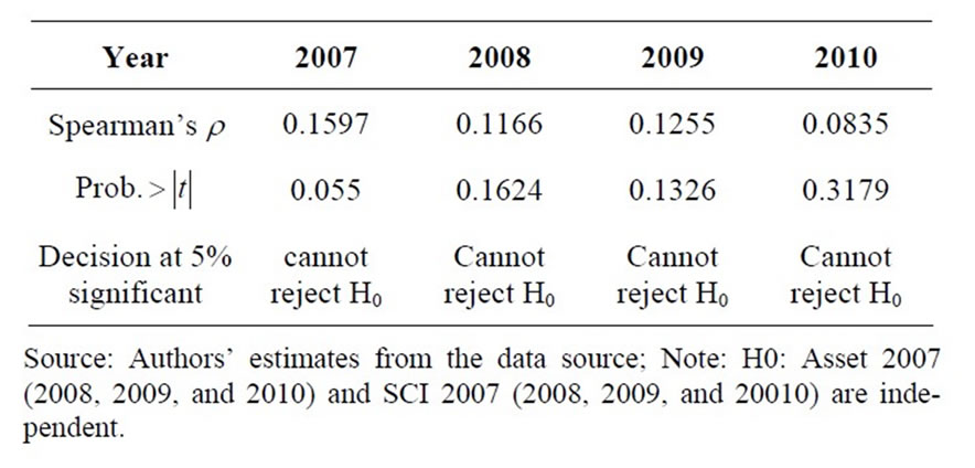
Table 11. Statistical Tests for the relation between banks’ total assets and super-efficiency from SCI model under CRS assumption using spearman’s test.
SBM and SCI models. To do so, we use:
1) Spearman Test for differences inefficiency score of the sample bank branches from SBM and SCI under the assumption of constant return to scale and variable return to scale;
2) Statistical tests for differences inefficiency score of the sample bank branches from SBM and SCI by Kendall’s tau; and
3) Two Banker’s asymptotic DEA efficiency tests for inefficiency differences between two different efficiency scores.
Before presenting the results of each test, we summary some estimated results from SBM model as the following. SBM models were estimated using the program DEASolver Software (2007). The super efficiency measures from the SBM model under the assumption of CRS and VRS for the sample bank branches in 2007, 2008, 2009, and 2010 are 0.6586, 0.6680, 0.6213 and 0.6597, respectively, while under the assumption constant return to scale for the sample bank branches in 2007, 2008, 2009, and 2010 are 0.749, 0.786, 0.764 and 0.781, respectively.
The estimated maximum super efficiency under the assumption of CRS for the sample banks in 2007, 2008, 2009, and 2010 are 1.3281, 1.4341, 1.5598 and 1.4815, respectively, and under the assumption of VRS for the sample banks in 2007, 2008, 2009, and 2010 are 1.318, 1.662, 1.725 and 1.719, respectively. The minimum value of super-efficiency under the assumption of CRS for the sample banks in 2007, 2008, 2009, and 2010 are 0.3555, 0.3793, 0.3229 and 03572, respectively, while under the assumption of VRS for the sample banks in 2007, 2008, 2009, and 2010 are 0.374, 0.404, 0.359 and 0.380, respectively. Full efficiency under CRS (superefficient measures are greater than or equal to one) estimated from SBM models in 2007, 2008, 2009 and 2010 are 20, 19, 17, and 19 of the 145 bank branches, respectively.
3.7. Tests for Differences Inefficiency Scores from Two Models
The two approaches were used to measure the superefficiency for the sample of the agricultural bank branches in Vietnam. SBM is based on the work of Tone (2002). The SCI model differs from Tone’s (2002) model in the object function used and classifies all the decision making units. To highlight the relation existing between super-efficiency series estimated from SBM and superefficiency series estimated from SCI approaches, as well as the relation between rank series from two models under the assumptions of CRS and VRS, we use Spearman correlation and Kendall’s tau-b. Results of the statistical tests on ranking efficiency between the sampled bank branches are shown in Tables 12 and 13. The Spearman rank correlation coefficients and Kendall’s tau-b coefficients between ranks from super-efficiency, estimated from SBM model SCI model, are positive and very high. Note that the sign of the coefficient of Kendall’s tau-b indicates the direction of the relationship, in which larger absolute values indicate stronger relationship.
The results of the above two test statistics provide us with two findings: 1) the correlations between estimated super-efficiency series from SBM model and SCI model are positively and highly significant level; and 2) the correlations between rank series estimated from those are strong.
Banker’s Test
To show differences between the average efficiency score of SBM and SCI models under the assumptions of variable return to scale and constant return to scale, we use two Banker’s asymptotic DEA efficiency tests. Tests have been used to test for inefficiency differences between two different efficiency scores.
1) The first test uses based on the assumption of the two inefficiencies (1 – qSBM and 1 – qSCI) from the SBM and SCI models that follow the exponential distribution.
The test statistic is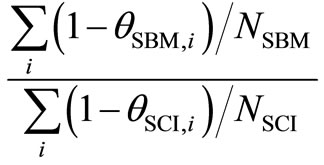 , evaluated relative to the F-distribution with (2NSBM, 2NSCI) degrees of freedom.
2) The second test is based on the assumption of the
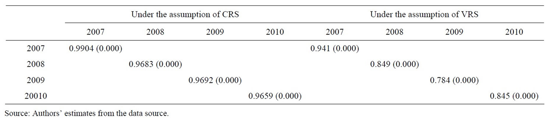
Table 12. Spearman rest for different inefficiency score of the sample banks from SBM and SCI under the assumption of constant return to scale and variable return to scale.
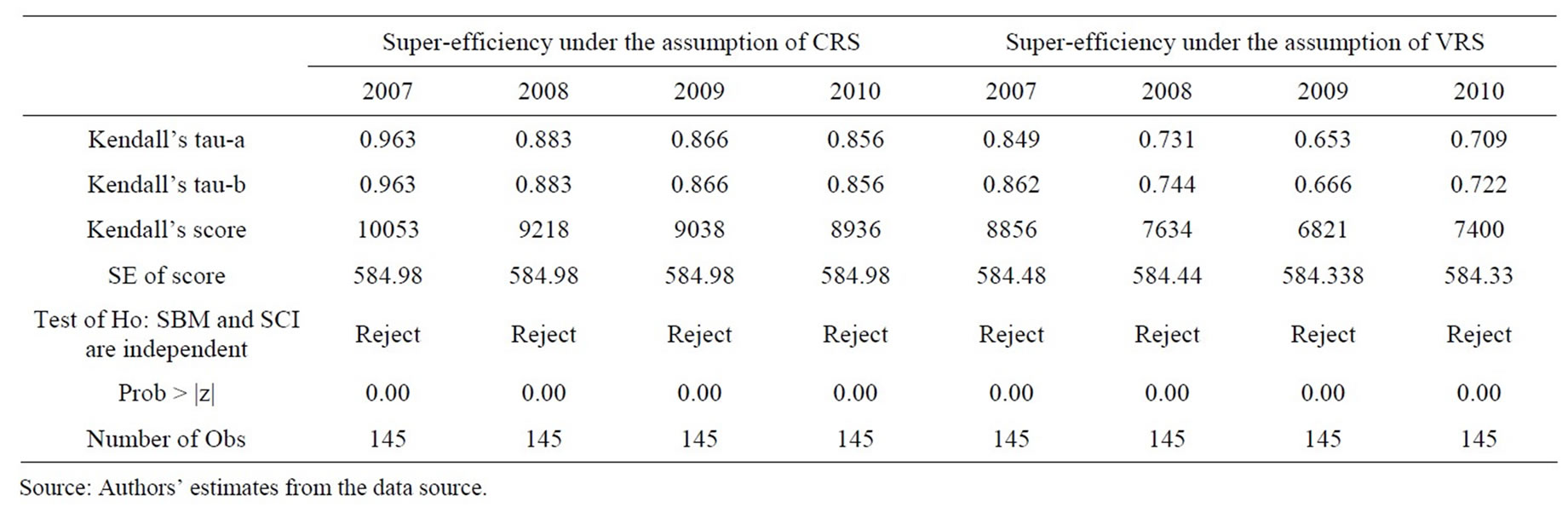
Table 13. Statistical tests for differences inefficiency score of the sample bank branches from SBM and SCI by Kendall’s tau.
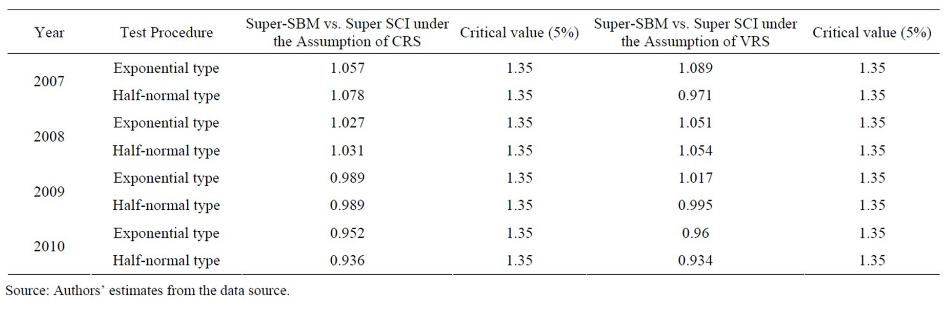
Table 14. Summary of efficiency difference test results.
two inefficiencies (1 – qSBM and 1 – qSCI) from the SMB and SCI models that follow the half-normal distribution.
The test statistic is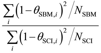 , evaluated relative to the F-distribution with (2NSBM, 2NSCI) degrees of freedom.
Table 14 presents the estimated results from Banker’s two asymptotic DEA tests for inefficiency estimated from each model and each year during 2007-2010. The estimated results show that there is no significant difference between the average efficiency score of SBM and SCI models.
4. Concluding Remarks
This paper presented the new approach to rank inefficient DMUs based on SBM. This model allowed the ranking of all inefficient DMUs and overcomes the disadvantages of infeasibility. The new approach was applied to rank super-efficient scores for the sample of 145 agricultural bank branches in Viet Nam during 2007-2010. By using the Spearman Rank Test, Kendall’s tau-b test and Bankers’ tests show that the ranks of the sampled bank branches based on the SBM and SCI approaches are highly correlated.
REFERENCES
- K. Tone, “A Slacks-Based Measure of Efficiency in Data Envelopment Analysis,” European Journal of Operational Research, Vol. 143, No. 1, 2002, pp. 32-41. doi:10.1016/S0377-2217(01)00324-1
- A. Charnes, W. W. Cooper and E. Rhodes, “Measuring the Efficiency of Decision-Marking Units,” European Journal of Operational Research, Vol. 2, No. 4, 1978, pp. 429-444. doi:10.1016/0377-2217(78)90138-8
- R. D. Banker, A. Charnes and W. W. Cooper, “Some Models for Estimating Technical and Scale Inefficiencies in Data Envelopment Analysis,” Management Science, Vol. 30, No. 9, 1984, pp. 1078-1092. doi:10.1287/mnsc.30.9.1078
- N. Adler, L. Friedman and Z. Sinuany-Stern, “Review of Ranking Methods in Data Envelopment Analysis Context,” European Journal of Operation Research, Vol. 140, No. 2, 2002, pp. 249-265. doi:10.1016/S0377-2217(02)00068-1
- P. Andersen and N. C. Petersen, “A Procedure for Ranking Efficient Units in Data Envelopment,” Analysis Management Science, Vol. 39, No. 10, 1993, pp. 1261- 1294.
- F. H. Liu and L. C. Tsai, “Ranking of DEA Units with a Set of Weights to Performance Indices,” The Fourth International Symposium on DEA, Aston University, 4-6 September 2004.
- F. H. Lotfi, M. Navabakhs, A. Tehranian, M. RostamyMalkhalifeh and R. Shahverdi, “Ranking Bank Branches with Interval Data—The Application of DEA,” International Mathematical Forum, Vol. 2, No. 9, 2007, pp. 429- 440.
- S. Li, G. R. Jahanshahloo and M. Khodabakhshi, “A Super-Efficiency Model for Ranking Efficient Units in Data Envelopment Analysis,” Applied Mathematics and Computation, Vol. 184, No. 2, 2007, pp. 638-648. doi:10.1016/j.amc.2006.06.063
- S. Mehrabian, M. R. Alirezaee and G. R. Jahanshahloo, “A Complete Efficiency Ranking of Decision Making Units in Data Envelopment Analysis,” Computational Optimization and Applications, Vol. 14, No. 2, 1999, pp. 261-266. doi:10.1023/A:1008703501682
- K. Tone, “A Slacks-Based Measure of Efficiency in Data Envelopment Analysis,” European Journal of Operational Research, Vol. 130, 2001, pp. 489-509. doi:10.1016/S0377-2217(99)00407-5
- C. A. Favero and L. Papi, “Technical Efficiency and Scale Efficiency in the Italian Banking Sector: A NonParametric Approach,” Applied Economics, Vol. 27, No. 4, 1995, pp. 385-395. doi:10.1080/00036849500000123
- D. C. Wheelock and P. W. Wilson, “Technical Progress, Inefficiency, and Productivity Change in U.S. Banking, 1984-1993,” Journal of Money, Credit and Banking, Vol. 31, No. 2, 1999, pp. 212-234. doi:10.2307/2601230
- G. Lang and P. Welzel, “Technology and Cost Efficiency in Universal Banking A ‘Thick Frontier’-Analysis of the German Banking Industry,” Journal of Productivity Analysis, Vol. 10, No. 1, 1998, pp. 63-84. doi:10.1023/A:1018346332447
- M. Asmild, J. C. Paradi, V. Aggarwall and C. Schaffnit, “Combining DEA Window Analysis with the Malmquist Index Approach in a Study of the Canadian Banking Industry,” Journal of Productivity Analysis, Vol. 21, No. 1, 2004, pp. 67-89. doi:10.1023/B:PROD.0000012453.91326.ec
- A. S. Camanho and R. G. Dyson, “Efficiency, Size, Benchmark and Targets for Bank Branches: An Application of Data Envelopment Analysis’,” Journal of Operation Research Society, Vol. 50, No. 9, 1999, pp. 903-915. doi:10.1057/palgrave.jors.2600792
- D. Hauner and S. Peiris, “Banking Efficiency and Competition in Low Income Countries: The Case of Uganda,” Applied Economics, Vol. 40, No. 21, 2008, pp. 2703-2720. doi:10.1080/00036840600972456
- D. C. Wheelock and P. W. Wilson, “New Evidence on Returns to Scale and Product Mix among U.S. Commercial Banks,” Journal of Money, Credit and Banking, Vol. 47, No. 3, 2001, pp. 653-674.
- T.-Y. Chen, “A Measurement of Taiwan’s Bank Efficiency and Productivity Change during the Asian Financial Crisis,” International Journal of Services Technology and Management, Vol. 6, No. 6, 2005, pp. 485-503. doi:10.1504/IJSTM.2005.007510
- N. K. Minh and G. T. Long, “Ranking Efficiency of Commercial Banks in Vietnam with Supper Slack-Based Model of Data Envelopment Analysis,” Proceeding of DEA Symposium, Seikei University, Tokyo, 2008.
- W. W. Cooper and K. Tone, “Measures of Inefficiency in Data Envelopment Analysis and Stochastic Frontier Estimation,” European Journal of Operational Research, Vol. 99, No. 1, 1997, pp. 72-78. doi:10.1016/S0377-2217(96)00384-0
- W. W. Cooper, L. M. Seiford and K. Tone, “Introduction to Data Envelopment Analysis and Its Use—With DEASolver Software and References,” Springer, New York, 2007.
- E. Fiorentino, A. Karmann and M. Koetter, “The Cost Efficiency of German Banks: A Comparison of SFA and DEA,” Discussion Paper Series 2: Banking Financial Studies, No. 10, Deutsche Bundesbank, 2006.
- L. Friedman, and Z. Sinuany-Stern, “Scaling Units via the Canonical Correlation Analysis and the Data Envelopment Analysis,” European Journal of Operation Research, Vol. 100, No. 3, 1997, pp. 629-637. doi:10.1016/S0377-2217(97)84108-2
- G. R. Jahanshahloo, L. F. Hosseinzadeh and M. Moradi, “Sensitivity and Stability Analysis in DEA with Interval Data,” Applied Mathematics and Computation, Vol. 156, No. 2, 2004, pp. 463-477. doi:10.1016/j.amc.2003.08.005
- L. M. Seiford and J. Zhu, “Infeasiblity of Super-Efficiency Data Envelopment Analysis Models,” Infor, Vol. 37, No. 2, 1999, pp. 174-187.
- T. R. Sexton, R. H Silkman and A. J. Hogan, “Data Envelopment Analysis: Critique and Extensions,” Measuring Efficiency: An Assessment of Data Envelopment Analysis, Vol. 1986, No. 32, 1986, pp. 73-105.
- Z. Sinuany-Stern, A. Mehrez and A. Barboy, “Academic Departments Efficiency via Data Envelopment Analysis,” Computers and Operations Research, Vol. 21, No. 5, 1994, pp. 543-556. doi:10.1016/0305-0548(94)90103-1
- Z. Sinuany-Stern and L. Friedman, “Data Envelopment Analysis and the Discriminant Analysis of Ratios for Raking Units,” European Journal of Operational Research, Vol. 111, No. 3, 1998, pp. 470-478. doi:10.1016/S0377-2217(97)00313-5
- A. M. Torgersen, F. R. Forsund and S. A. C. Kittelsen, “Slack-Adjusted Efficiency Measures and Ranking of Efficient Units,” Journal of Productivity Analysis, Vol. 7, No. 4, 1986, pp. 379-398. doi:10.1007/BF00162048