American Journal of Operations Research
Vol. 2 No. 2 (2012) , Article ID: 19953 , 6 pages DOI:10.4236/ajor.2012.22031
Optimal Promotion and Replenishment Policies for Profit Maximization Model under Lost Units
1P.G. Department of Statistics, Utkal University, Bhubaneswar, India
2Department of Business Administration, Utkal University, Bhubaneswar, India
3P.J. College of Management Technology, Biju Patnaik University of Technology, Bhubaneswar, India
Email: mscompsc@gmail.com, monalisha_1977@yahoo.com
Received December 28, 2011; revised January 30, 2012; accepted February 10, 2012
Keywords: Promotion; Deterioration; Inventory; Units Lost; Profit
ABSTRACT
Ever since its introduction in the second decade of the past century, the economic order quantity (EOQ) model has been the subject of extensive investigations and extensions by academicians. The physical characteristics of stocked items dictate the nature of inventory policies implemented to manage and control. The question is how reliable are the EOQ models when items stocked deteriorate one time. This paper introduces a modified EOQ model in which it assumes that a percentage of the on-hand inventory is wasted due to deterioration. There is hidden cost not account for when modeling inventory cost. We study the problem of promotion for a deteriorating item subject to loss of these deteriorated units. The objective of this paper is to determine the optimal time length, optimal units lost due to deterioration, the promotional effort and the replenishment quantity so that the net profit is maximized and the numerical analysis show that an appropriate promotion policy can benefit the retailer and that promotion policy is important, especially for deteriorating items. Furthermore crisp decision making is shown to be superior to crisp decision making without promotional effort cost in terms of profit maximization.
1. Introduction
Inventory management plays a crucial role in businesses since it can help companies reach the goal of ensuring prompt delivery, avoiding shortages, helping sales at competitive prices and so forth. To control an inventory system, one cannot be ignored demand since inventory is partially determined by demand, as suggested by [1] and [2] in many cases a small change in the demand pattern may result in a large change in optimal inventory decisions. A manager of a company has to investigate the factors that influence demand pattern, because customers’ purchasing behavior may be affected by factors such as promotional effort, units lost due to deterioration, quantity ordered, profit and so on. A subject in the area of inventory theory that has recently been receiving considerable attention is the class of inventory models with deterioration. With these models, the presence of retail inventory is assumed to have a motivating effect on the customer.
Many models have been proposed to deal with a variety of inventory problems. Comprehensive reviews of inventory models can be found in [3] and [4]. In previous deterministic inventory models, many are developed under the assumption that demand is either constant or stock dependent for deteriorated items. [5] dealt with the EOQ problem for deteriorating items with linear time dependent demand rate under inflation where shortages and discounts are allowed. [6] considered the effect of different market policies, e.g. the price per product and advertisement frequency on the demand of a perishable item. [7] analyzed two scenarios; the first considers TOD as a constant and the store manager may choose an appropriate value, while the second assumes that TOD is a random variable. [8] proposed the correct theory for the problem supplied with numerical examples. The most recent work found in the literature is that of [9] who extended his earlier work by assuming a time-varying demand over a finite planning horizon. [10] presented an EOQ inventory model for perishable items with a stock dependent selling rate. Unlike the work of [11] who studied the case of partial backlogging for deteriorating items. [12] studied an EOQ inventory model in which it assumes that the percentage of on-hand inventory wasted due to deterioration is a characteristic feature of the inventory conditions which govern the item stocked.
Furthermore, retailer promotional activity has become more and more common in today’s business world. For example, Wall Mart and Costco often try to stimulate demand for specific types of electric equipment by offering price discounts; clothiers Baleno and NET make shelf space for specific clothes items available for longer periods; McDonald’s and Burger King often use coupons to attract consumers. Other promotional strategies include free goods, advertising, displays and so on. The promotion policy is very important for the retailer. How much promotional effort the retailer makes has a big impact on annual profit. Residual costs may be incurred by too many promotions while too few may result in lower sales revenue. [13] discussed dynamic pricing, promotion and replenishment policies for a deteriorating item under permissible delay in payment. [14] studied the effects of inflation and time value of money on the replenishment policies of items with time continuous nonstationary demand over a finite planning horizon.
This study addresses the problem by proposing a continuous review inventory model under promotion by assuming that the units lost due to deterioration of the items. In this paper optimization has been studied for applying promotional effort cost with promotion constraint. The effect of deteriorating items on the instantaneous profit maximization replenishment model under promotion is considered in this paper. The market demand may increase with the promotion of the product over time when the units lost due to deterioration. In the existing literature about promotion it is assumed that the promotional effort cost is a function of promotion. [15, 16] studies profit maximization entropic order quantity model for deteriorated items with stock dependent demand where discounts are allowed for acquiring more profit. In this paper, promotional effort and replenishment decision are adjusted arbitrarily upward or downward for profit maximization model in response to the change in market demand within the planning horizon. The objective of this paper is to determine optimal promotional efforts and replenishment quantities in an instantaneous replenishment profit maximization model.
In recent years, companies have started to recognize that a tradeoff exists between product varieties in terms of quality, promotion of the product for running in the market smoothly. In the absence of a proper quantitative model to measure the effect of product quality and promotion of the product, these companies have mainly relied on qualitative judgment. This paper postulates that measuring the behavior of production systems may be achievable by incorporating the idea of retailer promotional effort in making optimum decision on promotion and replenishment with units lost due to deterioration. The major assumptions used in the above research articles are summarized in Table 1.
The remainder of the paper is organized as follows. In Section 2 assumptions and notations are provided for the development of the model. The mathematical formulation is developed in Section 3. The solution procedure is given in Section 4. In Section 5, numerical example is presented to illustrate the development of the model. The sensitivity analysis is carried out in Section 6 to observe the changes in the optimal solution. Finally Section 7 deals with the summary and the concluding remarks.
2. Assumptions and Notations
r: Consumption rate
tc: Cycle length
h: Holding cost of one unit for one unit of time.
HC(q): Holding cost per cycle
K: Setup cost per cycle
c: Purchasing cost per unit
α: Percentage of on-hand inventory that is lost due to deterioration
q: order quantity
q**: Modified economic ordering/production quantity (EOQ/EPQ)
q*: Traditional economic ordering quantity (EOQ)
j(t) : On-hand inventory level at time t
ρ: The promotional effort per cycle
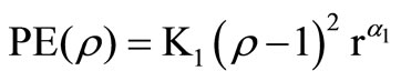
PE(r): The promotional effort cost,
PE(r) = K1(r – 1)2
where K1 > 0 and α1 is a constant π(q, p) are average
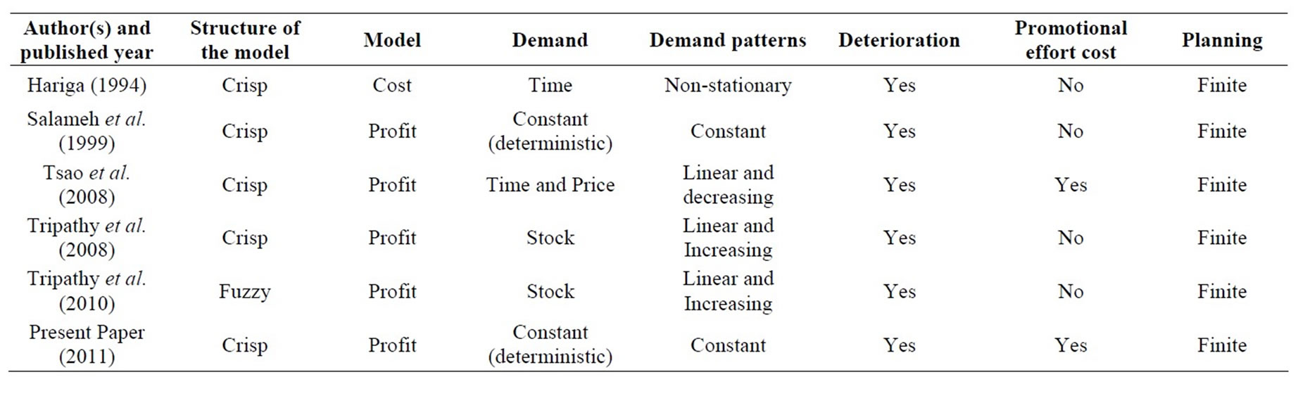
Table 1. Major characteristics of inventory models on selected researches.
profits per unit of producing q units per cycle in crisp strategy. π1(q, p) are the net profits per cycle in crisp strategy.
3. Mathematical Model
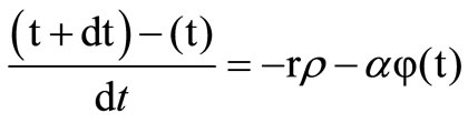
Denote j(t) as the on-hand inventory level at time t. During a change in time from point t to t + dt, where t + dt > t, the on-hand inventory drops from j(t) to j(t+dt). Then j(t+dt) is given as:
 (1)
(1)
Equation (1) can be re-written as:
 (2)
(2)
and dt ® 0, Equation (2) reduces to:
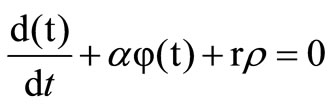 (3)
(3)
Equation (3) is a differential equation, solution is
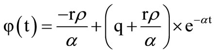 (4)
(4)
where q is the order quantity which is instantaneously replenished at the beginning of each cycle of length tc units of time. The stock is replenished by q units each time these units are totally depleted as a result of outside demand and deterioration. The cycle length, tc, is determined by first substituting tc into Equation (4) and then setting it equal to zero to get:
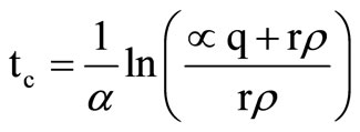 (5)
(5)
Equations (4) and (5) are used to develop the mathematical model. It is worthy to mention that as α approaches to zero,  approaches to
 . Then the total number of units lost per cycle, L, is given as:
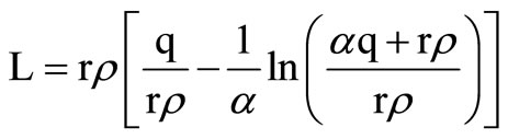 (6)
(6)
The total cost per cycle, TC(q), is the sum of the procurement cost per cycle, K + cq, the holding cost per cycle, HC(q), and the promotional effort cost per cycle, PE(r). HC (q) is obtained from Equation (4) as :
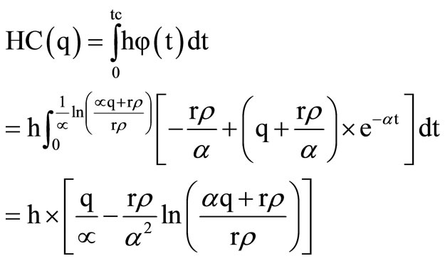 (7)
(7)
 (8)
(8)
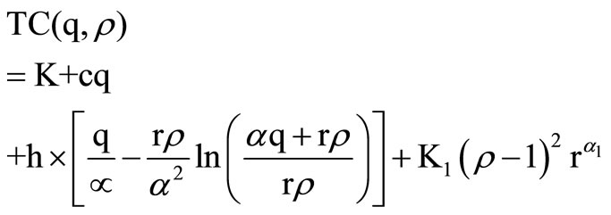 (9)
(9)
The total cost per unit of time, TCU(q,r), is given by dividing Equation (9) by Equation (5) to give:
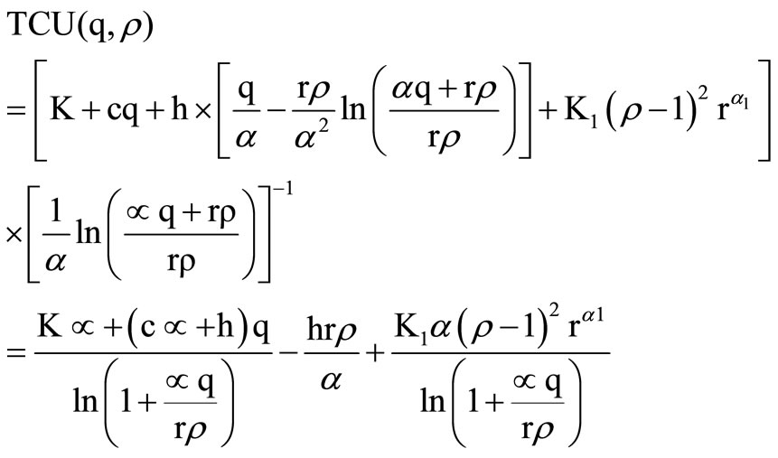 (10)
(10)
As α approaches zero and r = 1 Equation (10) reduces to TCU (q, ρ) = 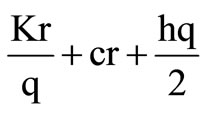
Whose solution is given by the traditional EOQ formula, . The total profit per cycle is p1(q, r).
 (11)
(11)
where L, the number of units lost per cycle due to deterioration, and TC(q, r) the total cost per cycle, are calculated from Equations (6) and (9), respectively. The average profit p(q, r) per unit time is obtained by dividing tc in p1(q, r). Hence the profit maximization problem is
Maximize p1(q, r),
 (12)
(12)
4. Solution Procedure (Optimization)
The optimal ordering quantity q and promotional effort r per cycle can be determined by differentiating Equation (11) with respect to q and r separately, setting these to zero.
In order to show the uniqueness of the solution in, it is sufficient to show that the net profit function throughout the cycle is jointly concave in terms of ordering quantity q and promotional effort r. The second partial derivates of Equation (11) with respect to q and r are strictly negative and the determinant of Hessian matrix is positive. We consider the following propositions.
Proposition 1. The net profit p1(q, r) per cycle is concave in q.
Conditions for optimal q
 (13)
(13)
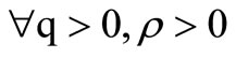
The second order partial derivative of the net profit per cycle with respect to q can be expressed as
 (14)
(14)
Since rr > 0 and  Equation (13) is negative.
Proposition 2. The net profit  (q, r) per cycle is concave in r.
Conditions for optimal r
 (15)
(15)
The second order partial derivative of the net profit per cycle with respect to r is
 .
.
Since K1 > 0, r > 0,  , we find that Equation (15) is negative.
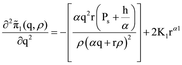
Propositions 1 and 2 show that the second partial derivatives of Equation (12) with respect to q and r separately are strictly negative. The next step is to check that the determinant of the Hessian matrix is positive, i.e.
 and
and 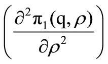 shown in Equations
(13 and 15) and
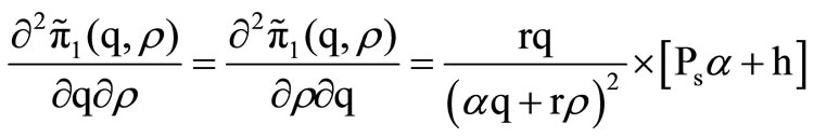 (16)
(16)
The average profit per unit time we have the following maximization problem.
Maximize  (q, r)
 (17)
(17)
The objective is to determine the optimal values of q and r to maximize the unit profit function. It is very difficult to derive the optimal values of q and r, hence unit profit function. There are several methods to cope with constraints optimization problem numerically. But here we use LINGO 13.0 software to derive the optimal values of the decision variables.
5. Numerical Example
Consider an inventory situation where K is Rs. 200 per order, h is Rs. 5 per unit per unit of time, r is 1200 units per unit of time, c is Rs. 100 per unit, the selling price per unit Ps is Rs. 125 and α is 5%, K1 = 2.0 and α1 = 1.0. The optimal solution that maximizes Equation (11) and  and
and  are determined by using LINGO 13.0 version software and the results are tabulated in Table 2.
6. Sensitivity Analysis
It is interesting to investigate the influence of α on retailer behavior. The computational results shown in Table 3 indicates the following managerial phenomena: when the percentage of on hand inventory that is lost due to deterioration α increases, the optimal replenishment quantity will decrease, the replenishment cycle length, the optimal total number of units lost per cycle and the optimal promotional effort will decrease respectively, simultaneously the optimal promotional effort cost and optimal total profit per unit of time will also decrease. The three-dimensional total profit per unit graph is shown in Figure 1. The results indicate that the total profit per unit is decreased as the percentage of on-hand inventory that is lost due to deterioration is increased as shown in Figure 2.
7. Conclusions
In this paper, a modified EOQ model is introduced which investigates the promotional effort parameter and it assumes that a percentage of the on-hand inventory is wasted due to deterioration as a characteristic feature and the inventory conditions govern the item stocked. This paper provides some useful properties for finding the optimal profit, promotional effort and ordering quantity with deteriorated units of lost sales. A new mathematical model is developed and numerical examples are provided to illustrate the solution procedure. The new modified EOQ model is numerically compared to the traditional
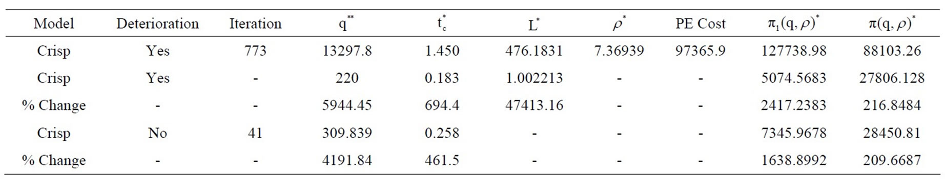
Table 2. Optimal values of the proposed model.
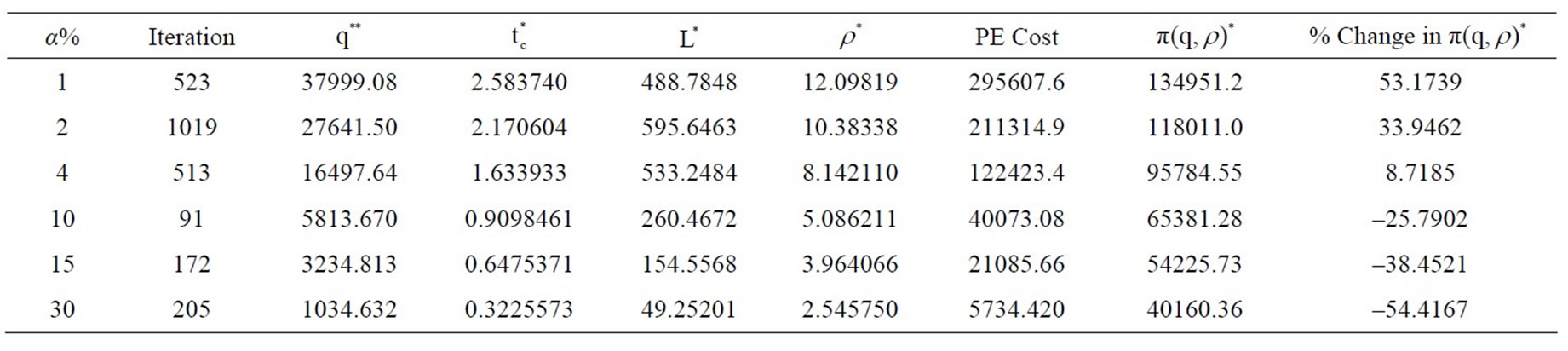
Table 3. Sensitivity analysis of α.
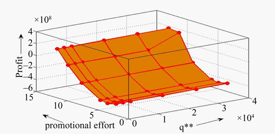
Figure 1. The total profit per unit time, 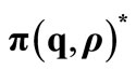 , q* and ρ*.
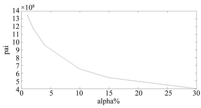
Figure 2. Graphical representation of total profit  and α%.
EOQ model. The economic order quantity and the net profit for the modified model,  were found to be more than that of the traditional,
  , i.e.
  and the net profit respectively. Finally, the promotion effort parameter effect was demonstrated numerically to have an adverse effect on the average profit per unit. Hence the utilization of promotional effort and units lost due to deterioration make the scope of the application broader.
The current work can be extended in order to incorporate the modified model with shortages are allowed and the consideration of multi-item problem. A further issue that is worth exploring is that of partial backlogging. Finally, few additional aspects that we intend to take into account in the near future are the applying dynamic pricing strategy through a new optimization model and stochastically of the quality of the products.
REFERENCES
- C. D. J. Waters, “Inventory Control and Management,” Wiley, Chichester, 1994.
- J. S. Osteryoung, D. E. Mc Carty and W. L. Reinhart, “Use of EOQ Models for Inventory Analysis,” Production and Inventory Management, Vol. 27, No. 3, 1986, pp. 39-45.
- F. Raafat, “Survey of Literature on Continuously Deteriorating Inventory Models,” Journal of Operational Research Society, Vol. 42, 1991, pp. 89-94.
- K. Jain and E. Silver, “A Lot Sizing for a Product Subject to Obsolescence or Perishability,” European Journal of Operational Research, Vol. 75, No. 2, 1994, pp. 287-295. doi:10.1016/0377-2217(94)90075-2
- S. Bose, A. Goswami and K. S. Chaudhuri, “An EOQ Model for Deteriorating Items with Linear Time-Dependent Demand Rate and Shortages under Inflation and Time Discounting,” Journal of the Operational Research Society, Vol. 46, 1995, pp. 775-782.
- S. K. Goyal and A. Gunasekaran, “An Integrated Production-Inventory-Marketing Model for Deteriorating Items,” Computers and Industrial Engineering, Vol. 28, No. 4, 1995, pp. 755-762. doi:10.1016/0360-8352(95)00016-T
- D. Gupta and Y. Gerchak, “Joint Product Durability and Lot Sizing Models,” European Journal of Operational Research, Vol. 84, No. 2, 1995, pp. 371-384. doi:10.1016/0377-2217(93)E0273-Z
- M. Hariga, “An EOQ Model for Deteriorating Items with Shortages and Time-Varying Demand,” Journal of the Operational Research Society, Vol. 46, 1995, pp. 398- 404.
- M. Hariga, “Optimal EOQ Model for Deteriorating Items with Time-Varying Demand,” Journal of the Operational Research Society, Vol. 47, 1996, pp. 1228-1246.
- G. Padmanabhan and P. Vrat, “EOQ Models for Perishable Items under Stock Dependent Selling Rate,” European Journal of Operational Research, Vol. 86, No. 2, 1995, pp. 281-292. doi:10.1016/0377-2217(94)00103-J
- H. M. Wee, “Economic Production Lot Size Model for Deteriorating Items with Partial Back-Ordering,” Computers and Industrial Engineering, Vol. 24, No. 3, 1993, pp. 449-458. doi:10.1016/0360-8352(93)90040-5
- M. K. Salameh, M. Y. Jaber and N. Noueihed, “Effect of Deteriorating Items on the Instantaneous Replenishment Model,” Production Planning and Control, Vol. 10, No. 2, 1999, pp. 175-180. doi:10.1080/095372899233325
- Y. C. Tsao and G. J. Sheen, “Dynamic Pricing, Promotion and Replenishment Policies for a Deteriorating Item under Permissible Delay in Payment,” Computers and Operations Research, Vol. 35, No. 11, 2008, pp. 35621-3580. doi:10.1016/j.cor.2007.01.024
- M. Hariga, “Economic Analysis of Dynamic Inventory Models with Non-Stationary Costs and Demand,” International Journal of Production Economics, Vol. 36, No. 3, 1994, pp. 255-266. doi:10.1016/0925-5273(94)00039-5
- P. K. Tripathy and M. Pattnaik, “An Entropic Order Quantity Model with Fuzzy Holding Cost and Fuzzy Disposal Cost for Perishable Items under Two Component Demand and Discounted Selling Price,” Pakistan Journal of Statistics and Operations Research, Vol. 4, No. 2, 2008, pp. 93-110.
- P. K. Tripathy and M. Pattnaik, “An Fuzzy Arithmetic Approach for Perishable Items in Discounted Entropic Order Quantity Model,” International Journal of Scientific and Statistical Computing, Vol. 1, No. 2, 2011, pp. 7-19.