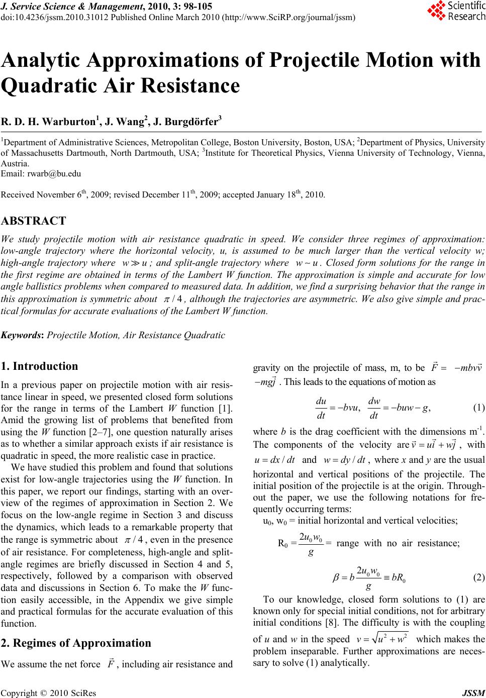J. Service Science & Management, 2010, 3: 98-105
doi:10.4236/jssm.2010.31012 Published Online March 2010 (http://www.SciRP.org/journal/jssm)
Analytic Approximations of Projectile Motion with
Quadratic Air Resistance
R. D. H. Warburton1, J. Wang2, J. Burgdörfer3
1Department of Administrative Sciences, Metropolitan College, Boston University, Boston, USA; 2Department of Physics, University
of Massachusetts Dartmouth, North Dartmouth, USA; 3Institute for Theoretical Physics, Vienna University of Technology, Vienna,
Austria.
Received November 6th, 2009; revised December 11th, 2009; accepted January 18th, 2010.
ABSTRACT
We study projectile motion with air resistance quadratic in speed. We consider three regimes of approximation:
low-angle trajectory where the horizontal velocity, u, is assumed to be much larger than the vertical velocity w;
high-angle trajectory where wu; and split-angle trajectory where wu. Closed form solutions for the range in
the first regime are obtained in terms of the Lambert W function. The approximation is simple and accurate for low
angle ballistics p roblems when compared to measured data. In additio n, we find a su rprising b ehavior tha t the ra nge in
this approximation is symmetric a bout /4

, although the trajectories are asymmetric. We also give simple and prac-
tical formulas for accurate evaluations of the Lambert W function.
Keywords: Projectile Motion, Air Resistance Quadratic
1. Introduction
In a previous paper on projectile motion with air resis-
tance linear in speed, we presented closed form solutions
for the range in terms of the Lambert W function [1].
Amid the growing list of problems that benefited from
using the W function [2–7], one question naturally arises
as to whether a similar approach exists if air resistance is
quadratic in speed, the more realistic case in practice.
We have studied this prob lem and found that solutions
exist for low-angle trajectories using the W function. In
this paper, we report our findings, starting with an over-
view of the regimes of approximation in Section 2. We
focus on the low-angle regime in Section 3 and discuss
the dynamics, which leads to a remarkable property that
the range is symmetric abou t /4

, even in the presence
of air resistance. For completeness, high-angle and split-
angle regimes are briefly discussed in Section 4 and 5,
respectively, followed by a comparison with observed
data and discussions in Section 6. To make the W func-
tion easily accessible, in the Appendix we give simple
and practical formulas for the accurate evaluation of this
function.
2. Regimes of Approximation
We assume the net force
F
, including air resistance and
gravity on the projectile of mass, m, to be
F

 mbvv


mgj

. This leads to the equations of motion as
,,
du dw
bvubuw g
dt dt

 (1)
where b is the drag coefficient with the dimensions m-1.
The components of the velocity arevuiwj

, with
/udxdt

and /wdydt

, where x and y are the usual
horizontal and vertical positions of the projectile. The
initial position of the projectile is at the origin. Through-
out the paper, we use the following notations for fre-
quently occurring terms:
u0, w0 = initial horizontal and vertical velocities;
R0 =00
2uw
g
= range with no air resistance;
00 0
2uw
bbR
g
  (2)
To our knowledge, closed form solutions to (1) are
known only for special initial conditions, not for arbitrary
initial conditions [8]. The difficulty is with the coupling
of u and w in the speed 22
vuw which makes the
problem inseparable. Further approximations are neces-
sary to solve (1) analytically.

Analytic Approximations of Projectile Motion with Quadratic Air Resistance 99
We consider three approximations aimed at linearizing
the speed according to the relative magnitudes of u and w:
low-angle trajectory (LAT) approximation,uw; high-
angle trajectory (HAT) approximation, wu; and
split-angle trajectory (SAT) approximation, uw, as,

22
,
,
2 ,
uifuwLAT
vuww ifwuHAT
uorw ifuwSAT











(3)
Each of the approximations will be discussed below,
with the emphasis on LAT that is important in practice
and in ballistics.
3. Low-Angle Trajectory (LAT) Approximation
3.1 The Trajectory
We assume in this case the horizontal velocity is on av-
erage much greater than the vertical velocity, uw.
This will be the case if the firing angle is small, a case
also discussed by Parker [9]. Here the speed may be ap-
proximated as vu  according to (3), so that the equa-
tions of motion in the LAT approximation are
2,.
du dw
bubuw g
dt dt
 (4)
One can solve for u first, after which w, x, and y can be
obtained. Hereafter, we will omit non-essential interme-
diate steps. The solutions may be verified by substitution
into the equations of motion . The so lutions are
00 0
/2 1
,,,
112
uwgt
uw gtabu
at at

 
 (5)
2
0
111
ln(1+ ),ln(1+ ).
242
g
gt
xatyw atgt
baaa

 


(6)
Equation 6 gives the trajectory in t he LAT approximation.
The trajectories computed from (6) are plotted in Fig-
ure 1 for three angles: 20o, 45o, and 70o. The initial speed
is 9.8 m/s for all angles. The drag coefficient is
1
0.1bm

.
For comparison, we also show the trajectory from
ideal projectile motion with no air resistance and the tra-
jectory from the solutions with the full 2 v air resistance,
Equation 1. We will simply refer to the former as the
ideal motion, and the latter as the fu ll solution.
The full solution is carried out by numerically inte-
grating the equations of motion with the full 2 v resis-
tance (1), using the Runge-Kutta method. (The two
curves labeled HAT and SAT in Figure 1 are discussed
in Sections 4 and 5.)
The agreement between the LAT approximation and
the full solutio n is good at 20o (nearly indistinguishable in
Figure 1(a)), and it becomes worse for larger angles. This
is as expected since the assumption was that LAT is valid
only at small angles. The range is much reduced compared
to the ideal motion. Air resistance in troduces in the traj ec-
tories a well-known backward-forward asymmetry. The
ascending part of the trajectory is shallower and longer,
and the descending part is steeper and shorter.
Figure 1. The trajectories for an initial speed of 09.8m/sv

and drag coefficient 1 0.1mb  at three firing angles, 20o
(a), 45o (b), and 70o (c). The labeled curves are (see text):
Full (thick solid line) - the numerical solution with the full
2
v resistance; LAT (solid line); HAT (dashed line, see Sec-
tion 4); SAT (dash-dotted line, see Section 5), Ideal (dotted
line) - motion without air resistance

Analytic Approximations of Projectile Motion with Quadratic Air Resistance 100
3.2 The Range and Height in Comparison with
Measurements
To find the range of the projectile we eliminate t from (6)
to obtain

02
0
exp(2)1 .
24
gx g
yw bx
au a

 

 (7)
The range, R, is the value of x when 0.y It satisfies

02
0
exp(2) 10.
24
gR g
wbR
au a

 

 (8)
This is a transcendental equ ation that until now had been
customarily solved numerically or graphically [9 ]. But as
we reported [1], equatio ns of this typ e can also be solved
analytically, with the results written in closed form in
terms of the Lambert W function.
The Lambert W function [10] is defined, for a given
value z, as the (inverse) function satisfying




exp .WzWz z (9)
Our discussions below refer closely to the properties
of this relatively “new” function. For readers unfamiliar
with this function, we give a brief review in the Appen-
dix. There the reader will also find some practical for-
mulas for evaluating W.
To solve for the range R in terms of W, (8) needs to be
rearranged in the form of (9) such that the multiplicative
prefactor to the exponential,

Wz, is the same as the
exponent. This can be achieved by following the steps in
[1]. The result is
1111
2exp 2exp,
1111
bR bR

 

 



(10)
with defined in (2). We identify from (9) and (10) that
 
111
2,or ,
121
11
exp
11
Wz bRRWz
b
z



 
 
 

 

 



(11)
This is the closed form expression for the range, R, in
the LAT approximation.
The height, H, can be obtained by maximizing y in (7),
and is given by

0
0
1ln 1+1 .
2
w
Hbu










 (12)
We compare in Table 1 measured range and height
data with calculations from Equations 11 and 12 for fir-
ing angles less than one degree. (The details of the cal-
culations are given in the next subsection.)
Table 1 shows that the measured data [11] and the cal-
culations agree well once the firing angle is above about
10 minutes of arc. The discrepancy between measure-
ment and theory is due to the uncertainty in the value b
(see Table 1 caption), and not the approximation itself.
Because the largest angle is still less than 1, higher order
corrections are negligible. The relative error for the
height is usually much larger than the relative error for
the range. This is probably due to the difficulty in accu-
rately measuring the relatively small height in this case.
The large errors in height and in range at the two small-
est angles need not cause concern. It is due to the combi-
nation of exceeding difficulty in determining the small
angle and the small height at the same time. Note that the
diameter of the projectile and the height are of the same
order of magnitude here. Overall, this example shows that
if a reasonable b can be obtained, the LAT approximation
should work well for low angle ballistics problems.
3.3 Analytic Properties of the Range
3.3.1 The Symmetry of Range in Firing Angle
The analytic Formula 11 enables us to immediately draw
several surprising conclusions on the general properties
of the range, R. Since z is a function of
 which depends
on the product


00 0
2uw sin

(0

is the firing angle),
we conclude that i) the range R is symmetric about /4

,
that is to say, two firing angles 1

and 2

will lead to
the same range if 11 /2



 (see the LAT curves in
Table 1. Measured and calculated results for a projectile of mass m = 9.7 g, diameter d = 0.76 cm, and muzzle velocity 823 m/ s.
The measured data are taken from [11]. Results are calculated from the LAT approximation (11,12). The drag coefficient b =
1.05x10-3 m-1 is determined from 2/bCd m  , where C = 0.15 is the recommended value [11], and  = 1.2 kg/m3 is the air
density
Firing Angle (min) 2 5 8 12 16 20 26 33 40 49
Measured 91 183 274 366 457 549 640 732 823 914
Calculated 76 177 265 367 456 534 636 738 826 923
Range, R (m)
Error, % 16 3.3 3.3 0.27 0.22 2.7 0.63 0.82 0.36 0.98
Measured 0.02 0.1 0.19 0.33 0.61 1.0 1.5 2.3 3.2 4.5
Calculated 0.011 0.068 0.17 0.36 0.62 0.93 1.5 2.3 3.2 4.5
Height (m)
Error, % 45 32 11 9.1 1.6 7.0 0.0 9.5 3.2 2.2

Analytic Approximations of Projectile Motion with Quadratic Air Resistance 101
Figures 1(a) and (c)); and ii) because W(z) is a mono-
tonic function, the maximum range occurs at /4

[12].
Remarkably, these properties i) and ii) with air resistance
in the LAT approximation are exactly the same as for
ideal projectile motion without air resistance.
Given initial conditions 0 u and 0 w, the range, R,
can be computed from (11). Since z is negative and W(z)
is multi-valued (see Appendix) for 0z＜, we have a
choice of the branches 0
W or 1 W. Comparing z in (11)
and (9) we identify one trivial solution, namely the pri-
mary branch,

01
1
Wz



(13)
This solution, although mathematically correct, is un-
physical because it gives a zero range when substituted
into (11). The physical choice must be 1 W. We note
that for linear resistance [1] the choices were the opposite,
where 0 W was the physical solution and 1 W the un-
physical one.
The range, R, calculated from (11) using 1 W

is
shown in Figure 2 as a function of the firing angle. It
clearly demonstrates that R is symmetric about, and
maximum at, /4

. Also shown in Figure 2, for com-
parison, are the ranges for ideal projectile motion with no
air resistance and with the full 2 v resistance.
Unlike the LAT case, the range of the full solution in
Figure 2 is not symmetric about /4

. It reaches maxi-
mum at an angle below /4

, a fact that is well known.
Figure 2. The range of projectile motion as a function of the
firing angle 0

. The initial speed is 0 v= 9.8 m/s and the
drag coefficient is b = 0.1 m-1. The LAT approximation
(solid line) is maximum at and symmetric about /4

, as is
the ideal motion (dash-dotted line). The range with the full
2
v resistance (dashed line) peaks before/4

, and is
asymmetric
The LAT range is in good agreement with the full solu-
tion for low firing angles as expected, up to around
/6

. Compared to the ideal case, the maximum ranges
in the LAT and the full solutions are substantially re-
duced, by about 40% for this particular set of parameters.
We note that the LAT approximation produces asym-
metric trajectories (Figure 1) but symmetric ranges. The
physical reason can be traced to two factors influencing
the range: the time of flight and the average horizontal
velocity, as discussed below.
3.3.2 The Time of Flight and the Average Velocity
The average horizontal velocity, u, and the time of
flight, T, are related by
.RuT (14)
The time of flight T can be obtained from (6) by set-
ting
x
R

, at tT

. Together with (11), this gives
 
00
exp111 1
exp1 .
21
bR
TWz
bu bu









 







(15)
The average horizontal velocity can be expressed from
(14) and (15) as
 
1
0111
1exp1 .
21 21
u
uWz Wz





 




 
 

 




(16)
Quantitatively, as the firing angle increases, the time
of flight T increases, but the average horizontal velocity
u decreases. However, before/4

, the increase in T
is more than the decrease in u so that the range as
governed by (14), increases. After /4

, however, the
opposite happens so that the range decreases. The sym-
metric range is a result of the balance between T and u.
3.3.3 The Range for Small and Large Air Resistance
In the limit of small air resistance, 0b, the dimen-
sionless parameter  will be small, 0

. The argu-
ment z to the W in (11) approaches 1/ze , and


1Wz (see Appendix). Using the properties of
W(z) and after some algebra (we leave the details as an
exercise to the interested reader), the first order correc-
tion to the range, R, in (9) is
000
22
11,0,
33
RRRbR b 
 
 
 
  (17)
where 0
R is the range of ideal projectile motion, 0b

.
For large air resistance, 1b and 1

. As

, 1/z

 according to (11). Using the as-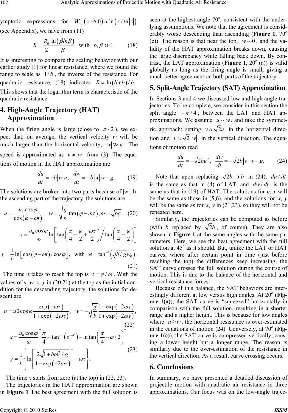

Analytic Approximations of Projectile Motion with Quadratic Air Resistance 102
ymptotic expressions for



10ln/Wz zlnz 
(see Appendix), we have from (11)

0ln with ,1.
2
ln
R
Rb
 

 (18)
It is interesting to compare the scaling behavior with our
earlier study [1] for linear resistance, where we found the
range to scale as 1/b, the inverse of the resistance. For
quadratic resistance, (18) indicates

ln ln/Rbbb.
This shows that the logarithm term is characteristic of the
quadratic resistance.
4. High-Angle Trajectory (HAT)
Approximation
When the firing angle is large (close to /2

), we ex-
pect that, on average, the vertical velocity w will be
much larger than the horizontal velocity, wu. The
speed is approximated as vw from (3). The equa-
tions of motion in the HAT approximation are
,.
du dw
bwubwwg
dt dt
 (19)
The solutions are broken into two parts because of |w|. In
the ascending part of the trajectory, the solutions are
 
0cos ,tan,.
cos
ug
uw bg
tb



 (20)
0cos ln tantan
42 242
u
x


 










10
1Incos/ cos,withtan/.yt bgw
b
 

 

(21)
The time it takes to reach the top is /t

 . With the
values of u, w, x, y in (20,21) at the top as the initial con-
dition for the descending trajectory, the solutions for de-
scent are





exp1 exp2
0cos ,,
1exp 21exp 2
g
uuw b







 
(22)


1 0
2
0
cos tanlntan/2
44
21 /
1ln .
1exp 2
t
u
xe
bg
yb










 






 







(23)
The time  starts from zero (at the top) in (22, 23).
The trajectories in the HAT approximation are shown
in Figure 1 The best agreement with the full solution is
seen at the highest angle 70o, consistent with the under-
lying assumptions. We note that the agreement is consid-
erably worse descending than ascending (Figure 1, 70o
(c)). The reason is that near the top, 0w, and the va-
lidity of the HAT approximation breaks down, causing
the large discrepancy while falling back down. By con-
trast, the LAT approximation (Figure 1, 20o (a)) is valid
globally as long as the firing angle is small, giving a
much better agreement on both parts of the trajectory.
5. Split-Angle Trajectory (SAT) Approximation
In Sections 3 and 4 we discussed low and high angle tra-
jectories. To be complete, we consider in this section the
split angle /4

, between the LAT and HAT ap-
proximations. We assume uw . and take the symmet-
ric approach: setting 2vu in the horizontal direc-
tion and 2vw in the vertical direction. The equa-
tions of motion read
2
2,2 .
du dw
bubw wg
dt dt

 (24)
Note that upon replacing 2bb in (24), /dudt
is the same as that in (4) of LAT, and /dwdt is the
same as that in (19) of HAT. The solutions for u, x will
be the same as those in (5,6), and the solutions for w, y
will be the same as for w, y in (21,23), so they will not be
repeated here.
Similarly, the trajectories can be computed as before
(with b replaced by 2b, of course). They are also
shown in Figure 1 at the same angles with the same pa-
rameters. Here, we see the best agreement with the full
solution at 45o as it should. But, unlike the LAT or HAT
curves, where after certain point in time (just before
reaching the top) the differences keep increasing, the
SAT curve crosses the full solution during the course of
motion. This is due to the balance of the horizontal and
vertical resistance forces.
Because of this balance, the SAT behaviors are inter-
estingly different at low versus high angles. At 20o (Fig-
ure 1(a)), the SAT curve is “squeezed” horizontally in
comparison with the full solution, resulting in a shorter
range and a higher height. This is because for low angles
where uw＞, the horizontal resistance is over-estimated
in the equations of motion (24). Conversely, at 70o (Fig-
ure 1(c)), the SAT curve is compressed vertically, caus-
ing a lower height but a longer range. The reason is
similarly due to the over-estimation of the resistance in
the vertical direction. As a result, curve crossing occurs.
6. Conclusions
In summary, we have presented a detailed discussion of
projectile motion with quadratic air resistance in three
approximations. Our focus was on the low-angle trajec-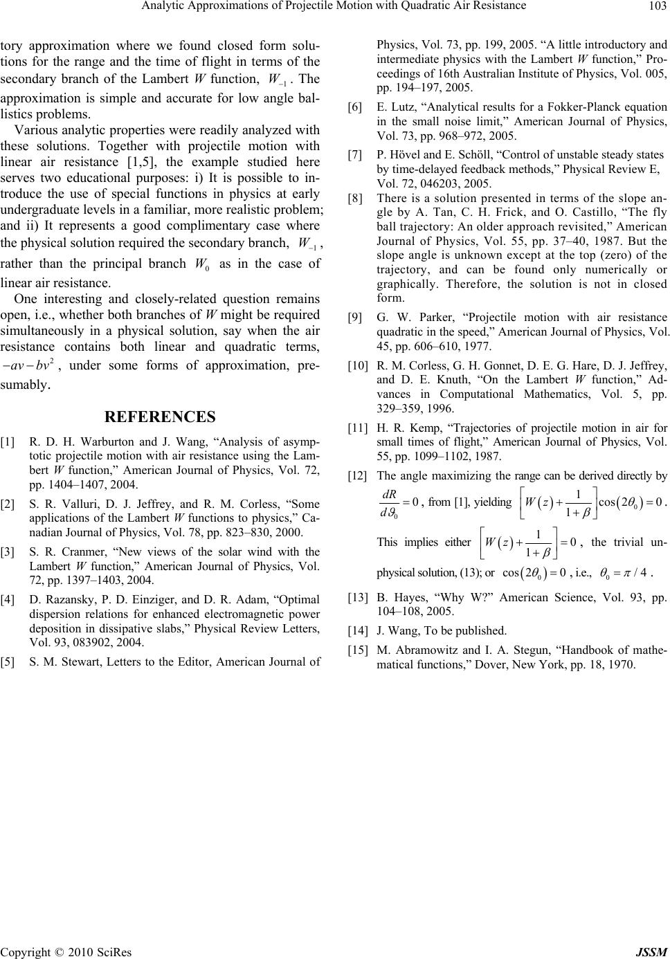

Analytic Approximations of Projectile Motion with Quadratic Air Resistance 103
tory approximation where we found closed form solu-
tions for the range and the time of flight in terms of the
secondary branch of the Lambert W function, 1 W

. The
approximation is simple and accurate for low angle bal-
listics problems.
Various analytic properties were readily analyzed with
these solutions. Together with projectile motion with
linear air resistance [1,5], the example studied here
serves two educational purposes: i) It is possible to in-
troduce the use of special functions in physics at early
undergraduate levels in a familiar, more realistic problem;
and ii) It represents a good complimentary case where
the physical solution requ ir ed the seco nd ar y b ran ch , 1
W

,
rather than the principal branch 0 W as in the case of
linear air resistance.
One interesting and closely-related question remains
open, i.e., whether both branches of W might be required
simultaneously in a physical solution, say when the air
resistance contains both linear and quadratic terms,
2
av bv , under some forms of approximation, pre-
sumably.
REFERENCES
[1] R. D. H. Warburton and J. Wang, “Analysis of asymp-
totic projectile motion with air resistance using the Lam-
bert W function,” American Journal of Physics, Vol. 72,
pp. 1404–1407, 2004.
[2] S. R. Valluri, D. J. Jeffrey, and R. M. Corless, “Some
applications of the Lambert W functions to physics,” Ca-
nadian Journal of Physics, Vol. 78, pp. 823–830, 2000.
[3] S. R. Cranmer, “New views of the solar wind with the
Lambert W function,” American Journal of Physics, Vol.
72, pp. 1397–1403, 2004.
[4] D. Razansky, P. D. Einziger, and D. R. Adam, “Optimal
dispersion relations for enhanced electromagnetic power
deposition in dissipative slabs,” Physical Review Letters,
Vol. 93, 083902, 2004.
[5] S. M. Stewart, Letters to the Editor, American Journal of
Physics, Vol. 73, pp. 199, 2005. “A little introductory and
intermediate physics with the Lambert W function,” Pro-
ceedings of 16th Australian Institute of Physics, Vol. 005,
pp. 194–197, 2005.
[6] E. Lutz, “Analytical results for a Fokker-Planck equation
in the small noise limit,” American Journal of Physics,
Vol. 73, pp. 968–972, 2005.
[7] P. Hövel and E. Schöll, “Control of unstable steady states
by time-delayed feedback methods,” Physical Review E,
Vol. 72, 046203, 2005.
[8] There is a solution presented in terms of the slope an-
gle by A. Tan, C. H. Frick, and O. Castillo, “The fly
ball trajectory: An older approach revisited,” American
Journal of Physics, Vol. 55, pp. 37–40, 1987. But the
slope angle is unknown except at the top (zero) of the
trajectory, and can be found only numerically or
graphically. Therefore, the solution is not in closed
form.
[9] G. W. Parker, “Projectile motion with air resistance
quadratic in the speed,” American Journal of Physics, Vol.
45, pp. 606–610, 1977.
[10] R. M. Corless, G. H. Gonnet, D. E. G. Hare, D. J. Jeffrey,
and D. E. Knuth, “On the Lambert W function,” Ad-
vances in Computational Mathematics, Vol. 5, pp.
329–359, 1996.
[11] H. R. Kemp, “Trajectories of projectile motion in air for
small times of flight,” American Journal of Physics, Vol.
55, pp. 1099–1102, 1987.
[12] T he a n gl e m axim izing t he range can be derived directly by
0
0
dR
d


, from [1], yielding
 
0
1cos 20
1
Wz






.
This implies either

10
1
Wz






, the trivial un-
physical solution, (13); or

0
cos 20  , i.e., 0/4



.
[13] B. Hayes, “Why W?” American Science, Vol. 93, pp.
104–108, 2005.
[14] J. Wang, To be published.
[15] M. Abramowitz and I. A. Stegun, “Handbook of mathe-
matical functions,” Dover, New York, pp. 18, 1970.

Analytic Approximations of Projectile Motion with Quadratic Air Resistance 104
Appendix
1. The Lambert W function
In this appendix, we briefly summarize some relevant
elements of the Lambert W function. The reader can find
an extensive review in [10]. In lieu of the growing inter-
est in this function in the physics community [2–7], we
also present several practical formulas for the evaluation
of the W function.
The Lambert W function as defined by (9) is generally
complex-valued. For our purpose we are interested in the
real-valued W(x), namely the principal branch 0
W, and
the secondary branch 1 W. The two branches are shown
in Figure 3.
The be havio rs of 0 W and 1 W

for small and large x are
  
2
01 0
00ln,ln.
ln ln
x
x
Wxxx WxWx
x
x


 
 
 
 
(A.1)
2. Evaluation of W
During the course of our study, we were unable to find in
the literature simple and practical algebraic expressions
for evaluating W over the whole range, and for embed-
ding it in our code. We therefore devised several readily
usable approximate formulas given here for this purpose.
It should give the interested reader a good starting point
in using this function.
W is not (yet) available on a calculator like some ele-
mentary functions. It is debatable whether it should be
elevated to the status of an elementary function. (See [13]
for an enchanting account.) However, one can easily im-
plement it on a programmable calculator with the formu-
las given here. The accuracy is at least 8 digits, in fact it
is usually much better.
Figure 3. The Lambert W function for real argument x. The
two real branches are the principal branch 0 W (solid line),
and the secondary branch 1 W (dashed line). The branch
point is at 1
x
e  where 1W


1) W in the Regular Regions
We first give the formulas optimized in the regular re-
gions. Owing to space limitations, we will explain the
methods used elsewhere [14]. The general form of the
expressions is


0, 1rWxCrP  (A.2)
where C is a constant and


rP is the Padé approxi-
mant defined as

234
01 234
234
123 4
r.
1
aarararar
Pbr brbrbr

  (A.3)
The expansion variable, r, is related to the independent
variable, x. We give in Table 2 the constant C, the vari-
able r, and the coefficients i a andi b. To utilize the ta-
ble, locate which function and region to use, then evalu-
ate (A.2) with the corresponding C, r, i a, and i b.
2) W in the Asymptotic Regions
Both 0 W and 1 W

have the same form in the asymp-
totic regions








 

2234
0, 11234
2
2
12 3
23
4
1,
ln /
ln,ln ,
ln 1
1/ 2,12/6,186/ 24,
1 225824/120.
Wxqqqrarararar
pq
xx
pqr
xpq
aaqaqq
aqqq
 
 

 
 


 
 
(A.4)
This expression (A.4) should be used for 0 W in the re-
gion


2.2,x

 and for 1 W in
 
0.12,x . Note
that it is the subtle difference in p, namely,


ln/ ln
x
x
for 0 W and


ln/ln-
x
x



 for 1
W that automatically
selects the correct branch.
3) W with a Little Programming
If the reader wishes to calculate W with arbitrary preci-
sion, one can use Newton’s rule [15] which, for a given x,
is the root, w, to


exp 0fwwwx

. The root-
finding process is as follows: Starting with an initial
guess, 1 w, the successive iterations, n w, approach rap-
idly to the true value as


2
1
exp ,1,2,3...
1
nn
n
n
wxw
wn
w



 (A.5)
It only remains to determine the initial guess, 1 w. One
way to choose 1
w is

Analytic Approximations of Projectile Motion with Quadratic Air Resistance 105
Table 2. The approximate formulas for the evaluation of W with (A.2) and (A.3). Spaces are inserted in the coefficients for
readability. For optimal precision, all the digits should be used
Function 0
W 1 W
Region 
1,0.16xe 

 


 0.16,0.32x

 0.32,2.2x

1,0.12xe 

 

Const. C -1 0 0.3906 4638 -1
Variable r

2ln ex
x


ln 3
x

2ln ex
0
a 1 1 0.2809 0993 -1
1
a -0.8040 7820 4.674 4173 0.1116 7016 -0.8178 4020
2
a 0.2802 9706 6.577 4227 0.0 3529 1013 -0.2889 3422
3
a -0.0 4785 3103 2.730 6731 0. 00 5498 1613 -0.0 5003 8980
4
a 0.00 3355 7735 0.1057 7423 0.000 4245 7974 -0.00 3566 1458
1
b -0.4707 4486 5.674 4173 0.1389 8485 0.4845 0686
2
b 0.0 9560 4321 10.75 184 0 0.0 7995 0768 0.0 9965 4140
3
b -0.00 6612 4586 7 .637 5538 0.00 4515 2166 0.00 7066 1014
4
b 0.7961 1402x10-5 1.539 0142 0.000 6368 7954 0.5596 5023x 10-5


10
10
11
1.5
ln 1.5
ln -0
x
if exW
wxif xW
x
if exW








＜
＜＜
＜
(A.6)
It can be shown [14] that (A.5) with the seed from (A.6)
always converges to the correct branch 0 W or 1 W

. Th e
convergence is fast, usually to machine accuracy in a few
iterations.
Summarizing, accurate values for 0 W and 1 W

over
all regions of x can be found by using Table 2 plus (A.4)
for fixed precision (8 digits or better), or (A.5) and (A.6)
for arbitrary precision.