Journal of Modern Physics
Vol.07 No.12(2016), Article ID:70136,21 pages
10.4236/jmp.2016.712139
Electromagnetic-Energy Flow in Anisotropic Metamaterials: The Proper Choice of Poynting’s Vector
Carlos Prieto-López, Rubén G. Barrera
Instituto de Física, Universidad Nacional Autónoma de México, México

Copyright © 2016 by authors and Scientific Research Publishing Inc.
This work is licensed under the Creative Commons Attribution International License (CC BY).
http://creativecommons.org/licenses/by/4.0/


Received 22 June 2016; accepted 23 August 2016; published 26 August 2016
ABSTRACT
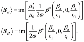
We study the controversy about the proper determination of the electromagnetic energy-flux field in anisotropic materials, which has been revived due to the relatively recent experiments on negative refraction in metamaterials. Rather than analyzing energy-balance arguments, we use a pragmatic approach inspired by geometrical optics, and compare the predictions on angles of refraction at a flat interface of two possible choices on the energy flux:  and
and . We carry out this comparison for a monochromatic Gaussian beam propagating in an anisotropic non- dissipative anisotropic metamaterial, in which the spatial localization of the electromagnetic field allows a more natural assignment of directions, in contrast to the usual study of plane waves. We compare our approach with the formalism of geometrical optics, which we generalize and analyze numerically the consequences of either choice.
Keywords:
Poynting Vector, Eikonal, Electromagnetic-Energy Flux, Anisotropic Metamaterials, Geometrical Optics

1. Introduction
The location of electromagnetic energy is an elusive subject that has been under discussion since the beginning of electrodynamics [1] . Even in the case of electrostatics, one can write at least two different expressions for the energy density of a fixed distribution of charges ( [2] , p. 21). In one of them, the energy density is proportional to the charge density itself, thus located wherever the charge density is different from zero; in the other one, it is proportional to the square of the electric field generated by the charge distribution, thus located in all space, both inside and outside the volume occupied by the charge distribution. On the side of electrodynamics, the am- biguity is even greater. The energy-balance equation in vacuum involves the time derivative of energy density of the electromagnetic field, given in terms of the squares of the electric and magnetic fields and the divergence of the Poynting vector; this vector is defined as proportional to the cross product of the electric and magnetic field and it gives the magnitude and direction of the energy flux ( [3] , sec. 61). Since the balance equation for energy conservation requires only the divergence of the Poynting vector, this vector field is not uniquely defined and it is always possible to add to it an arbitrary vector field with zero divergence. Furthermore, it is also possible to redefine both the Poynting vector and the expression for the energy density, in such a way as to fulfill correctly the balance equation [4] - [10] ( [11] , ch. 27.5). This freedom leads to an unsurmountable ambiguity about the location of electromagnetic energy and direction of the electromagnetic-energy flux. Nevertheless, it has been argued that the law of conservation of energy does not stand by itself, that there are also conservation laws for linear and angular momentum, and they have to be examined together. For example, in vacuum, the relationship between the Poynting vector (energy-flux field) and the electromagnetic linear-momentum density, together with the conservation of angular momentum, restricts the freedom of choice for the mathematical expression of the Poynting vector, and it has been even claimed that these restrictions remove the ambiguity altogether [12] [13] .
The problem of the location of energy and the correct expression for the energy flux in the presence of materials acquires additional intricate subtleties related to the description of the energy-exchange mechanism between fields and matter [14] [15] . First, let us recall that the formulation of macroscopic electromagnetic phenomena is commonly achieved by the introduction, besides the macroscopic electric field  and magnetic induction field
 , of two other fields: the displacement field
  and the magnetic intensity
 , or, equi- valently, the polarization and magnetization fields:
  and
and . In relation to the physical interpretation of these fields, a problem arises about an issue that has been discussed for more than a century: how to establish if
  or
or  represents the “real” magnetic field, that is, the one that comes after an averaging process of the magnetic field generated by the microscopic components of a given material. There are even carefully argued assertions by W. Thomson that the magnetic field inside the material is not even properly defined ( [16] and references therein). The choice in this issue has definite consequences in the energy-balance equation―also known as Poynting’s theorem―when extended to the case where materials are present. As we will discuss briefly in Section 2, this is specially important if we want to separate the total energy density into a component stored in the fields and a component stored or dissipated within the material.
Furthermore, in the more general case when the electromagnetic response is linear but not instantaneous, it necessarily depends on frequency and it is dissipative. In this case it is not possible to separate the energy density into material, field and absorption contributions. But even in low-dissipation frequency bands, the correct expression for the Poynting vector (energy flux) depends on the explicit form of the energy-balance equation. Also, in relation to the freedom of choice of Poynting’s vector and the restrictions imposed by other conservation laws: linear and angular momentum, one has to recall that unlike in vacuum, in the presence of material media the relation between Poyting’s vector and the linear-momentum density of the electromagnetic field is still controversial [17] . There have been at least two proposals for the correct mathematical expression for the linear-momentum density: one given originally by M. Abraham ( ) [18] and the other one given originally by H. Minkowski (
 ) [19] , being these two choices the source of a persisting debate about either their correctness or their physical interpretation ( [20] , and references therein). There are also more drastic claims assuring that the macroscopic electromagnetic field within a material is actually a non-physical quantity, and that real measurement devices do not really measure the energy flux given by the Poynting vector [21] .
Here we will not analyze all different aspects of these longstanding and sometimes subtle questions. We will rather concentrate only in two different proposals for the mathematical expression of the Poynting vector , whose choice has created controversy even in recent years [22] - [30] . One given by
 , which is the commonly used in literature and the one that appears in most textbooks and the other by
 , where we use SI units and
  is the so-called magnetic permeability of vacuum. On the one hand, the first expression is proposed by arguing that with this choice the boundary conditions on
  and
and  assure no accumulation of energy at any interface between two materials ( [3] , sec. 61). On the other hand, some authors state that a correct analysis of the energy-balance equation in materials should lead to an expression for the energy flux given, not by
 , but rather by
 , and that the accumulation of energy at the interface causes no conceptual problem because in magnetic materials the source of energy dissipation at the interface are the induced surface currents [22] [28] [31] . It is appropriate to recall that these proposals have been recently re-examined, due somewhat to the current work done around the phenomenon of negative refraction in metamaterials [32] - [38] .
In this paper, rather than discussing the energetic balance in the material, we propose to look at the con- troversy from the perspective of geometrical optics in an extremely pragmatic approach, based on the fact that the energy flux is not only used to calculate energy balances, but also to quantify light intensity and its direction of propagation. To watch the refraction of a laser beam on a transparent prism is a very common and intuitive experience, in which one could very naturally speak about the “location” of the energy and the direction and “bending” of the energy flux. In contrast, in the idealized case of a plane wave the energy is on the average evenly distributed over all space, and it is therefore unlocalized, making it impossible to use such “intuitive” arguments as above.
For the two fields  and
and  in discussion, however, a comparison in these terms is not illuminating in usual isotropic materials, since their directions coincide. But for anisotropic materials, their directions need not to coincide, and this effect can be particularly important in anisotropic metamaterials, that can exhibit negative refraction, in which this difference becomes critical. Although negative refraction can be obtained also in isotropic metamaterials, anisotropic metamaterials have an important advantage: the conditions for obtaining negative refraction in them are much less restrictive.
Having all this in mind, we tackle the problem by constructing a “ray” of light in order to see how does it refract at an interface between vacuum and an anisotropic metamaterial. One can find different definitions of ray in geometrical optics, for example, one, as a line in the direction of the gradient of the eikonal [3] [39] , another, simply as a continuous line along the direction of the energy flow [40] , and still another one that defines ray merely as a beam [41] . Here we will adopt a rather intuitive picture of a ray by regarding it as a very narrow beam. Then we use continuum electrodynamics to calculate the spatial location of the reflected and refracted beams, together with the energy flow according to the two proposals in question. Then we compare―among other things―their directions with the direction of the beam.
The structure of the paper is as follows: in Section 2 we compare, for each energy-flux proposal, possible interpretations of the energy-balance equations and the terms involved in them; then in Section 3 we present a brief introduction of the electromagnetic properties of anisotropic uniaxial metamaterials with emphasis on the refraction of plane waves at a flat interface; we later state in Section 4 some basic properties of 2D mono- chromatic electromagnetic fields, on which we build our analysis, and make a comparison with the formalism of geometrical optics, which we extend in Section 5. In Section 5.1 we particularize the results and concepts of these two previous sections to a Gaussian beam; we study some its main characteristics, and sketch how to calculate its refraction, to finally display and analyze the corresponding results of the numerical simulations. Section 6 is devoted to our conclusions.
2. Poynting’s Theorem
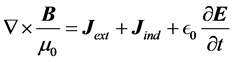
In this section we present briefly the energy-balance equations for the two energy-flux proposals to establish the differences in interpretation of the terms appearing in them. We start with the macroscopic Maxwell’s equations and regard the presence of the material as given by the charge and current densities induced by an external electromagnetic field produced by external sources. Maxwell’s equations, in SI units, can be then written as
 (1)
(1)
 (2)
(2)
 (3)
(3)
 (4)
(4)
where  and
and  are the charge and current densities that are sources of the external field that excites the material, while
  and
and  denote the macroscopic averages of the charge and current densities that are induced within the material. Here
  denotes the macroscopic electric field while
  denotes the macroscopic magnetic field obtained as the macroscopic average of the microscopic magnetic field. Let us recall that regrettably
  is also called magnetic induction. Then we divide
  into two terms,
 (5)
(5)
where 1)  denotes the induced conduction (“free”) plus polarization current densities and 2)
  denotes a divergence-free current density that behaves as the source of magnetization. Here
  and
and  are the usual polarization and magnetization material fields. Induced-charge conservation is also assumed, that is,
 (6)
(6)
By substituting Equation (5) into Ampère-Maxwell’s law (4) and using the induced charge conservation (6), one can write Equations (1) and (4) as
 (7)
(7)
 (8)
(8)
which together with Equations (2) and (3) form the complete set of the four macroscopic Maxwell’s equations. Here
 (9)
(9)
is called the displacement field, while
 (10)
(10)
is called the magnetic intensity or simply the H field.
If one now calculates  and uses the macroscopic Maxwell’s equations together with the defini- tions of
  and
and , as given by Equations (9) and (10), one can write
 (11)
(11)
that takes the mathematical form of a conservation law for the energy, and one can interpret  as an energy flux and
  as the energy density stored in the electromagnetic field. Notice that we write the expression of the energy density in terms of
  and
and , because we regard then as the fundamental “bare” fields. Nevertheless, since in our calculations below we deal with time averages of monochromatic fields in lossless materials, this choice will have no consequences in the final result. Here
  denotes the power supplied by the external current, while the last term in the right hand side should correspond to the temporal rate of change of the electric and magnetic energy density either stored or dissipated within the material. It is appropriate to point out that in the presence of dissipation the stored energy density within a material is not a well-de- fined concept since it cannot be written as a time derivative ( [3] , sec. 61).
Following the same procedure as above, one can also write the following equation:
 (12)
(12)
In this expression one identifies as the energy flux, and although the last term in the right hand side can be written as
 , and it could be naturally identified as the power dissipated by the induced currents, such identification contradicts the one given in Equation (11). Furthermore, the difference between
  and
and  is
is , and let us recall that
  has been identified in certain circumstances, as a “hidden” momentum, that is, a mechanical momentum conveyed by and within the magnetic material. Here c denotes the speed of light.
We will not discuss further the physical interpretation of the terms that appear in the energy-conservation laws given in Equations (11) and (12); we now rather construct the conceptual and mathematical framework to analyze the energy transport in the refraction of a beam of light at the interface between vacuum and an anisotropic metamaterial. The advantage of dealing with anisotropic metamaterials rather than with crystals, is that in crystals the anisotropy of the electromagnetic response is fixed by the crystalline structure and cannot be changed, while in metamaterials this degree of anisotropy, as well as the signs of the response, can be tailored through the fabrication process.
3. Uniaxial Metamaterials
As discussed above, we will be dealing with anisotropic uniaxial metamaterials. These are characterized by electric and magnetic response tensors  and
and , respectively. We will assume that they have a common anisotropy axis (the z-axis) thus they are simultaneously diagonalizable, with components
 ,
,  , and analogously with the components of
 . We also assume that we will be working on a frequency band in which the material is transparent, that is, at frequencies where all the components of these response tensors can be regarded as real (i.e., negligible absorption). Furthermore, the premise that we are dealing with metamaterials allows us to choose not only over a wide spread of values for the tensorial components, but also their sign.
We will now introduce notation and summarize some of the properties that we will use in this paper; their derivation can be found, for example, in [42] . First we recall that an uniaxial metamaterial sustains two elec- tromagnetic plane-wave modes, which we will call e and m, and refer to them generically as . Each mode is characterized by a given frequency
  and a corresponding wavevector
 . In the m -mode, the electric field
  es orthogonal to
  while in the e-mode the
  field is orthogonal to
 . We will also refer generically to the diagonal components of either
  or
or  as
as  and
and , when referring to the m or to the e mode, respectively; and in terms of these we define the anisotropy factor
 , that is,
  and
and . The anisotropy factor quantifies the degree of anisotropy of the response; its deviation from unity gives us an idea of how anisotropic the response of the medium is.
The dispersion relations of these modes can be put in terms of , the magnitude of the wavevector of
  mode,
mode,  , and the wavenumber in vacuum
 . Assuming the wavevector lies in the xz plane, these can be written as
 (13)
(13)
Note that  would be the index of refraction of the system in the absence of anisotropy (
 ).
).
Finally, it is important to say that, in this medium, the field  is not, in general, parallel to
  for a monochromatic plane wave. Let us call
  the amplitude of the
  field for
  and the amplitude of the electric field for
 , and the subscripts i, r and t will denote the incident, reflected and transmitted fields, respectively. Then, the field
  is, in average,
 (14)
(14)
so both vectors will only be parallel when there is no anisotropy of the corresponding mode ( ).
).
Refraction of Plane Waves
Let us consider a plane interface between vacuum and the uniaxial metamaterial, set this interface perpendicular to the optical axis of the metamaterial and fix the z-axis along this direction. Then assume that a plane wave, with its wavevector in the xz plane, impinges from vacuum into the metamaterial. One can immediately see that if the incident wave is p-polarized ( perpendicular to
 ) only the e mode is excited, while if it is s-polarized (
 perpendicular to
 ) only the m mode is excited; while
  remains in the xz plane, and thus, there are separate “refraction laws” for
  and
and .
.
Now we look at the reflection and transmission of plane waves in the presence of uniaxial metamaterials, defined as  and
and ;
;  as
as  for
for  (p-polarization) and
  for
for  (s-polarization); and using boundary conditions at the interface, we can write
 (15)
(15)
where .
.
In terms of these definitions and basic concepts, we now summarize some interesting features of the refraction of plane waves on uniaxial metamaterials. A derivation of all these results can be found in [42]
1) The angle  formed by
  and
and , in terms of the incidence angle
 , is
, is
 (16)
(16)
2) The angle  formed by
  and
and , again in terms of the incidence angle
 , is given by
 (17)
(17)
and we call this the refraction angle.
3) The refraction of  is towards the interface if
  and away the interface if
 . The projection
of  over
over  also has the sign of
 .
.
4) The sign of refraction is determined by the sign of .
.
5) The refraction angle, as a function of the incidence angle, is an increasing function if  and decreasing if
 .
.
6) Whenever , there exists a critical angle (equal for
  and
and ), given by
 .
.
7) The critical angle has an inverse behavior in the case , in the sense that, for angles lower than the critical, there is no propagating wave transmitted, but for all angles higher that the critical, there is propagating transmission.
8) There exist critical angles for both polarizations.
9) There is low variation of the refraction angle for .
.
10) In the particular case when , the reflectance is constant for all angles.
Note especially, on relation with negative refraction, some less restrictive features of these materials due to their anisotropy, for example, the sign of the projection of  over
over  is no longer tied to the sign of the refraction angle, since it is determined by only one parameter; also, there can be propagating transmitted waves even if the “refractive index” is purely imaginary.
With respect to point 3, it is important to note that this refraction problem has a mathematical ambiguity arising from the fact that the dispersion relation (13) is quadratic, and thus two possibilities for  are admitted (while
  is fixed by boundary conditions). This is solved by noting that, independently of the physical interpretation of the field
 , the continuity of the parallel components of
  and
and  lead to the continuity of its normal (z) component across the interface. Besides, since
  is, by construction, positive on the incidence medium, it has to be positive on the refraction medium, which together with Equation (14), tells us that
  and
and  should have the same sign. Here
  is a unit vector along the z axis.
4. 2D Monochromatic Fields
In this work we will be dealing, for simplicity, with the refraction of monochromatic two-dimensional beams, that nevertheless keep most of the physics behind the phenomenon of refraction of actual three-dimensional beams. We consider first an arbitrary two-dimensional monochromatic electric field, defined as a superposition of plane waves in the xz plane,
 (18)
(18)
where re denotes real part. In a given medium, this will be a solution to Maxwell's equations if  as a function of
  is given by the dispersion relation of the electromagnetic waves in this medium. For example, for an isotropic medium with refractive index n, this relation is:
 . As it can be seen, this field does not depend on the y coordinate implying translational invariance along this direction. A plot of the magnitude of this field in the xz plane will mimic a projection of a three-dimensional monochromatic field.
We can view this superposition as a series of plane waves traveling along different directions and with different amplitudes, these determined by the function . In general, this superposition includes not only propagating waves, but also inhomogeneous waves, that is, plane waves with a complex wavevector
  whose amplitudes decay along
  and propagate with its planes of constant phase perpendicular to
 .
.
Recalling now that the magnetic, displacement, and  fields linked to the electric field
of a plane wave of wavevector  and frequency
 , can be written as
 (19)
(19)
it is immediate to write the corresponding monochromatic fields associated to the electric field given in Equation (18), as
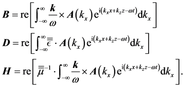 (20)
(20)
For s-polarization, the amplitudes  in (18) can be written as
 . It is then convenient to define
 (21)
(21)
thus in terms of  the electric field in (18) becomes
 (22)
(22)
Note that if we denote ,
,  , then
 (23)
(23)
and the same is valid for  replacing
  with
with  in the integrand. Now, since
  and
and  one can write, for s-polarization, the magnetic, displacement, and
  fields in Equation (20) in a most convenient and succinct way:
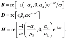 (24)
(24)
For p polarization, one can write an expression for the  field, analogous to the one for the electric field in Equation (18), as
 (25)
(25)
where
 (26)
(26)
with the following corresponding expressions for the displacement, electric and magnetic fields,
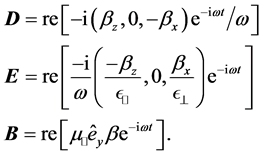 (27)
(27)
It is important to note that the linear superposition of plane waves, as the one given in Equation (18) can be
also written as , where the exponent
  has been pulled out of the integral leaving
a factor that is a function only of position. Since in the calculation of the energy densities and energy flux we will be dealing with bilinear products of the form  it is convenient to introduce time averages of these bilinear quantities, because the measuring devices cannot simply follow time variations of the order of
 . Since the factor multiplying
  is only a function of the position, we will frequently deal with products of this type. If we denote with a ' the real part of a complex numbers and with '' its imaginary part, the product above is written as
 . Now, if one takes the time average over periods much longer than
  one gets,
 (28)
(28)
where we have used  to indicate time average and the * denotes complex conjugate.
For example, using Equations (22) and (28), the time average of  for s-polarization is
 (29)
(29)
Also, from Equations (22) and (24) one can easily calculate , and its time average by using again equation (28). One gets, for s-polarization,
 (30)
(30)
Note that this result is general and does not depend on the constitutive relations. On the other hand, for  we do not have any such general expression, but we can calculate one for the special case of anisotropic metamaterials; using Equations (22) and (24), one gets, again for s-polarization,
 (31)
(31)
which clearly differs in direction from .
.
Finally, regarding to the energetic consequences of the choice of energy flux, note that, taking the divergence of  and calling
  to the second partial derivatives of
 , we get
 (32)
(32)
Since , in isotropic media with real refractive index n, this quantity
has the value  and, therefore, the divergence will be zero. But in a medium with a different dispersion relation-for instance, an anisotropic one-this will be nonzero. Since we don’t have a general expression in terms of
  for
for , it is not possible to calculate its divergence in an arbitrary case, but it is possible to do it in the special case of the anisotropic metamaterials, for which we get, with analogous calculations in s-polarization,
 (33)
(33)
which, in view of the dispersion relation (13), and following the same reasoning as before with , is identi- cally zero in mediums where
  is real. Thus, in the cases of isotropic and anisotropic media for an s-polarized monochromatic field, we have that
  does not predict any local loss or gain of energy within the material, while
  does predict it in the anisotropic metamaterial.
5. Geometrical Optics and Light Beams
As we already mentioned in the introduction and in the section concerning the refraction of plane waves, the energy-flux vector (Poynting’s vector) is used, besides the calculation of electromagnetic-energy transport, in determining the “detectable” direction of refraction of plane waves, over the direction given by the angle of refraction of the wavevector. Although in many cases they do coincide, their difference in direction is specially critical in the phenomenon of negative refraction. In our pragmatic approach we will look at the refraction of rays―defined as narrow beams―and then calculate the two expressions for the energy flux:  and
and , and compare their direction with the actual direction of the beam.
The first question is how to define the location of the beam in order to visualize it. The first idea could be perhaps to identify it with the transmitted energy flux and visualize it by plotting the transmittance, which is what one usually associates as the measurable quantity in optics experiments. The problem with such definition is that the value of the transmittance depends on the definition of the energy flux, which would lead us to a circular argument. Also, let us recall that the transmittance is proportional to the energy flux perpendicular to the interface, as if the detection of the transmitted power would be accomplished only along the perpendicular direction and not along the direction of the beam. Thus, we choose to look instead at the energy density, which in the absence of dissipation is proportional to , and then take the direction of the beam as the direction of the energy flux.
In the search of a criterion to determine how a monochromatic field refracts, one may require to define the direction of propagation of the field. At this respect, we derived the following result which we find interesting, and, to our knowledge, unnoticed yet. Let us start considering the simplest case of an isotropic, homogeneous, non-magnetic medium in which  (
( ), and assume that the monochromatic field is s- polarized. Note that the average of this field given in (30) is proportional to
 , and also that
 (34)
(34)
We recognize in  the phase
  of the complex function
 ; therefore, by com- bining Equations (34), (30) and (29), one can write
 (35)
(35)
Since the electric field in Equation (22) can be also written as , we conclude that in a
homogeneous, isotropic, non-magnetic medium, the time average of the field  of a monochromatic, s-polarized field, points in the direction of the maximum change of the phase of the electric field. This exact result establishes a connection between the propagation of an arbitrary monochromatic field (which can be, in particular, a localized one) and the formalism of geometrical optics, by generalizing the concept of eikonal to such field, in the sense of a function whose gradient yields the direction of the “ray”. Notice that the concept of eikonal is usually introduced when there is slow spatial variation of the amplitude function of the electric field ( [3] , sec. 85), ( [39] , ch. 8), but here we impose no restriction on the spatial part.
Going a little bit further, note that the dependence on the material in the expressions for the electric field  in Equation (22) and the magnetic field
  in Equation (24) comes only through the specific form of
 , that requires the dispersion relation of the specific material in the performance of the integral in Equation (21). Therefore, Equation (35) is valid regardless the optical properties of the material, simply because its derivation is independent of the particular structure of
  (see Equations (30) and (34)). This means that in any material, the field
  of an arbitrary s-polarized monochromatic field, points in the direction of the gradient of phase of the corresponding electric field.
This same result does not hold for all materials while regarding the energy flux as given by . For instance, for an uniaxial magnetic medium excited with s-polarized light, the average of
  is given by (31) which differs markedly from the expression for the average of
  given in Equation (30). But even if the material is isotropic but has magnetic absorption,
  and
and  will also differ in direction: one can see this by replacing
  and
and  in Equation (31) by
  and recalling that
 ,
,
 (36)
(36)
The real part of  is
is , which can be expressed as
 , so one
can write
 (37)
(37)
One can see that the first term in the right hand side points along the direction of the gradient of phase of the electric field as in the case of a homogeneous nonmagnetic material, but now, due to absorption, the field  acquires a component in the direction of the maximum change of intensity. One can see this result as a generalization to arbitrary monochromatic fields in s-polarization, of the characteristics of propagation of inhomogeneous plane waves in absorbing media. In this latter case the inhomogeneous wave is proportional to
  where the planes of constant phase travel along
  while the planes of constant amplitude decay along
 .
.
Nevertheless, the very general result that for any monochromatic electromagnetic field and for any material the direction of  coincides with the gradient of the phase of the electric field, makes
  a very tempting choice for the energy flux. Note that the result is true even for absorbing media.
The analogous result for p polarized light might not be as obvious, but is also quite interesting. Using the expressions for the fields given in Equations (25) and (27) one can write,
 (38)
(38)
Without magnetic absorption, both fields are parallel, even in anisotropic media. Moreover, none of them has the property of pointing in the direction of maximum change of the phase of . The field that has this property for p-polarization is the field
 :
:
 (39)
(39)
where we have written . These results may be in principle unexpected, but perhaps it can
be mathematically clarified by the fact that Maxwell's equations in regions free of external sources together with the constitutive relations are invariant under the interchange of  and
and  and
and . One might think that this third field should be added to the other two options under consideration, however, in view of the equivalence of the
  in s-polarization and
  in p-polarization, we only need to take care of the two first-mentioned cases, fortunately. In the next subsection we adopt our definition of ray as a narrow Gaussian beam.
Gaussian Beam
We now use the results for 2D monochromatic fields to construct a localized beam. We start by regarding an s-polarized beam localized along the z-axis, and impose a boundary condition over the magnitude E of the electric field at , that defines its shape. This boundary condition requests that in the plane
 , E has a Gaussian profile of width w, that is,
 (40)
(40)
From Equation (22) we get that . This means that
  can be iden-
tified as the spatial Fourier transform of , and the condition of E being real only means that
 . Then
 (41)
(41)
Thus, the electric field in any point at any time is given by
 (42)
(42)
This is a 2D Gaussian beam, confined in the x direction and extended along the z direction. Regarding its composition as a superposition of plane waves, note that the plane wave corresponding to wavevector  has the dominant amplitude; we call this wave the main mode, and its corresponding vector the main wavevector. Now, given any other plain-wave component with wavevector
 , there is a corresponding plane wave component with the same amplitude and opposite x component, and therefore a wavevector
 ; their sum always “points” in the direction of the main wavevector. This gives the z axis a special geometrical role of symmetry, and thus we find natural to call it the axis of the beam and to say that the beam is propagating in the z direction. Naturally, the profile of
  is also Gaussian, and in it this symmetry is traduced on an invariance under the change of z by
  or x by
 . This also gives the point
  a special geometrical location (exactly at the center of the beam’s waist), and we call it the center of the beam.
We will be plotting , which is given exclusively in terms of the function
  defined in Equation (45), so, from now on, we will abuse lightly from the notation and refer to the function
  as “the beam”.
We are interested in the refraction of an incident beam from vacuum to an anisotropic metamaterial, but with an arbitrary angle of incidence , We assume the interface is located at the plane
  and then we write down the expression of the beam in Equation (42), in a rotated system of coordinates
  that we will call the incidence system, in which the
  plane is rotated an angle
  with respect to the xz plane, leaving y invariant. Then
 (43)
(43)
and the relationship between these two coordinate systems is given by
 (44)
(44)
Replacing these rotated variables in Equation (43) we get the following expression for the incident beam on the  system,
 (45)
(45)
where the axis of the beam lies along the line . We can recognize
  and
and  as the quantities in the exponent, that are in parenthesis multiplying x and z, respectively. So we can think of this Gaussian beam as a superposition of plane waves with wavevectors
  (on the unrotated system)―where
  and
and 
are related through the dispersion relation―and amplitudes given by  (given in the rotated system).
Note that the center of the beam remains in the same position.
Given the incident field in Equation (45) and setting the location of the uniaxial metamaterial in , we now describe the computation of the electric field of the refracted and reflected beams. The axis of the incident beam subtends an angle
  with the z axis. We then refract the beam by refracting mode by mode, under- standing that by refraction of the mode we only mean using Maxwell’s equations to propagate the plane-wave mode towards the anisotropic metamaterial, without any consideration about the direction of energy flow. This means that a transmitted mode with wave vector
 , obeys the dispersion relation in the metamaterial keeping its x component continuous at the interface.
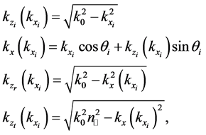
To this purpose, we follow the next steps to refract and reflect a given mode of the incident beam:
1) For a given mode-characterized in the integral by  -calculate the corresponding
  component using the dispersion relation in vacuum:
 .
.
2) From the resultant wave vector , obtain its component parallel to the interface
  by
by
rotating it as required in Equation (44).
3) Calculate the z-component of this mode by using the dispersion relation in the corresponding medium (vacuum or metamaterial), and assigning
a) a negative sign for the reflected mode.
b) the sign of 
 for the transmitted mode, as explained above.
4) Multiply the amplitude of this mode by the transmission or reflection coefficient in Equation (15), as a function of the parallel (x-component) of the wavevector.
To summarize this, we have, in terms of
 (46)
(46)
the expressions for the reflected and transmitted fields:
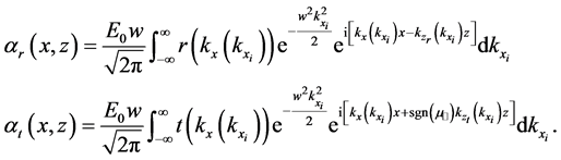 (47)
(47)
It is worth to note that the reflected and transmitted beams are―due to the presence of the transmission and reflection amplitudes inside these integrals―not Gaussian beams any more. This makes them no longer have the symmetries of the incident beam. Thus, we need a criterion to define the direction of propagation of the transmitted and reflected beams. It seems plausible to define this direction tracing a circle of radius r from the center of the beam, and, for each r, look for the local maximum of . The curve formed of all this points will serve for terms of this specific beam as the “geometrical ray”. Perhaps this will be more clear when we show the beam in the following subsection.
It is convenient for both, calculations and analysis, to express the above relations regarding the composition of the beam in terms of dimensionless quantities. For this, we define  which is a measure of the waist of the beam relative to the wavelength of the modes in vacuum;
 , a dimensionless version of the wave vector, relative to the wavenumber in vacuum;
 , a measure of the position in units of the waist of the beam; and
 , the dimensionless complex amplitude.
In terms of these quantities, Equation (43) can be expressed equivalently as,
 (48)
(48)
Naturally, there are analogous dimensionless quantities for the reflected and transmitted beams (47). In terms of  and of the dimensionless version of the components of
 :
:  and
and  relative to vacuum, we also define
 (49)
(49)
which are dimensionless measures of the averages of  and
and , respectively.
We will now take a look at the results of numerical simulations of the refraction of the Gaussian beam. These computations were obtained through a custom c program and plotted in gnuplot with a little help of bash. The source code can be freely downloaded from our page1. For the plotting, we present here some numerical results with effective-medium anisotropic parameters from actual metamaterial experimental reports [43] and [44] .
The first material is a laminate metamaterial (LM) made up of a succession of sheets of silver and silica. We took the effective properties at 400 nm of the seven-layered version. This material does not respond mag- netically but has an electrical anisotropic permittivity. Its parallel component for this wavelength is  while the orthogonal component is
 . We ignored the imaginary components of the tensor in agree- ment with the main assumptions presented above. The results should be presented for p-polarization, but, in order to make a more straight comparison with the second material described below, we switch to s polarization and interchange
  for
for .
.
The second metamaterial is a split ring resonator (SRR). SRR’s were the first constructed metamaterials in which negative refraction was observed. In order to obtain an isotropic response they were built by placing equal resonators on the cells of a cubic lattice. This SSR omitted the isotropization process, placing the resonators in parallel sheets, thus obtaining an uniaxal anisotropic metamaterial. At a microwave frequency of 1.8 GHz the effective properties (again, ignoring the imaginary part) are  and
and , while at 2.0 GHz we have
  and
and . Note that for both, the SRR and the LM we have
 .
.
Some points to take into account when looking at the results of the simulations are:
1) Due to the dimensionless representation we are using, the units of length in the plots are the width of the beam. Therefore, a same plot with larger larger units of length is equivalent to a thinner beam and vice-versa. In all the figures presented here, we use a parameter . This means that the actual beam waist depends on the beam frequency; for example, for yellow light with a wavelength of
  in vacuum, the waist would be of approximately 28 mm, a really slim beam. Of course, we suppose that assume the beam is sufficiently wide with respect to the metamaterial components so as to retain the validity of the effective- medium theory and―of course―macroscopic electrodynamics.
2) The fields  and
and  are scaled differently. The use of large values of
  implies very different sizes of
  and
and , which makes it difficult to visualize them, so, for each given plot, they are rescaled in a way such that their maximum sizes are equal.
First of all and in order to clarify the idea we have been discussing about the refraction of a light beam, we show in Figure 1 the plot of a beam seen from “far away”. This is the picture of a beam impinging from vacuum at an angle  over an isotropic material with the refractive index of diamond (2.4). We can see the incident, reflected and transmitted beams. And, as we said, the concentration of the field in this beam allows a natural definition of a direction.
The symmetry of the beam described in the preceding section makes us expect that in some approximation the propagation of the beam is represented by the propagation of the main mode. Thus, we also indicate the direction of  and
and  for the main mode; since for a plane wave this directions are constant, we plot lines in such directions passing through the center of the beam.
We present the results for the refraction of the beam at a vacuum-LM interface in Figure 2 and Figure 4; and at a vacuum-SRR interface in Figure 5 and Figure 6. The plots include the energy-density patterns, the field lines of  and
and  and the directions of these two fields for the main mode. For the same setup as in Figure 2 we display in Figure 3 the divergence of
  given by Equation (32); we omitted to show the divergence of
  since, as proved before, it is identically zero, and decided not to include the divergence corresponding to the other figures since they turn out to be very similar to Figure 4.
There are some features of these results that we would like to remark:
1) Unlike Figure 1, all the figures show an interference pattern between the incident and the reflected beam.
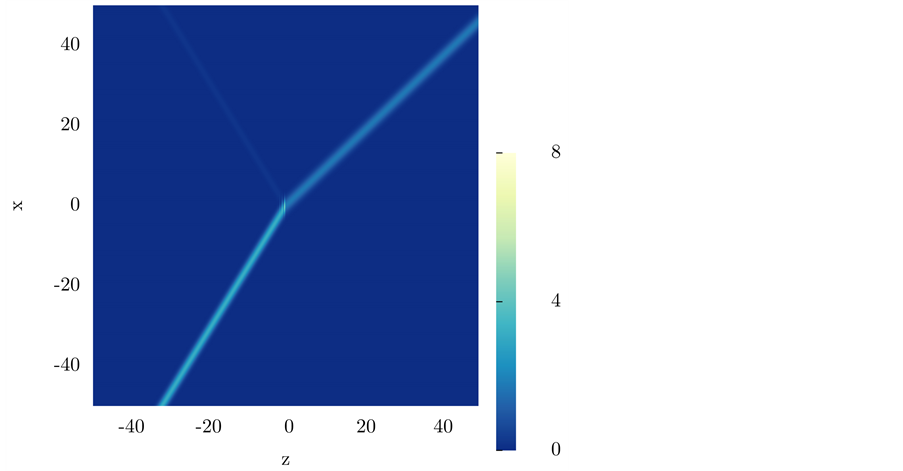
Figure 1. Gaussian beam refraction and reflection from vacuum into diamond, when viewed from far away.
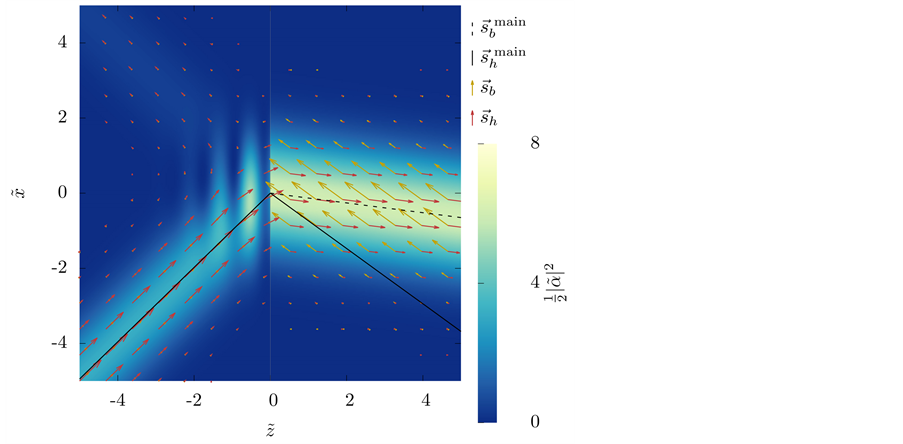
Figure 2. Refraction of the Gaussian beam from vacuum towards the LM for 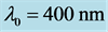 and
and . We plot a measure of the energy density (in the color map), the
  and
and  fields (as vector fields), and the direction of the
  and
and  for the main mode of the beam (as lines).
A stationary field is established by this interference, just as it happens in the interference between incident and reflected plane waves on an interface, case in which the interference term is a function exclusively of z. This characteristic is somewhat preserved in the beam although it is highly localized (these plots are just windows of  widths of the beam).
2) Away from the interference zone, the direction of both  and
and  fields does not vary appreciably . In particular in the transmitted beam, both fields seem to preserve their direction over all the plotted region. In the interference zone they bend continuously from the direction of incidence to the direction of reflection. When
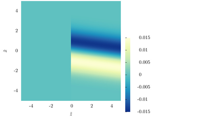
Figure 3. Divergence of  for the Gaussian beam of Figure 2.
Figure 4. Refraction of the Gaussian beam from vacuum towards the LM for  and
and . We plot a measure of the energy density (in the color map), the
  and
and  fields (as vector fields), and the direction of the
  and
and  for the main mode of the beam (as lines).
viewed from far away, we would only notice an abrupt change in direction from the incidence to the refraction angle.
3) As expected, both  and
and  coincide in direction in vacuum. Their size is numerically the same, but, as explained before, we used a different scale for the magnitude of each field.
4) The “rays” of  and
and  are―with the exception of the interference zone―parallel to the
  and
and  fields, respectively. If there is any deviation, it cannot be appreciated by only looking at the figure.
5) In all the simulations that we displayed, the line traced by the local maxima of  described before coincided―without noticeable difference―with the line corresponding to
 .
.
6) The magnitude of both  and
and  is larger on the more “intense” parts of the beam, and decreases when getting away from it.
7) In Figure 2 and Figure 4 the transmitted beam seems more intense than the incident beam.
And last, perhaps the most important observations:
8) For all cases,  has a small but quantifiable divergence along the transmitted beam. In all cases, it is negative in some regions and positive in others . A plot of this is displayed in Figure 3. This means that if
  is interpreted as an energy flux, there is energy flowing out in some regions of the beam, and energy flowing in in other regions of the beam , which requires a justification in physical terms.
9) Some of the basic refraction properties of the propagation of plane waves in uniaxial metamaterials re- ferred in Section 3 are preserved in the case of the beam: a) Negative refraction is obtained when  is nega- tive, as in Figure 2, Figure 4 and Figure 6. b) The projection of
  over
over  (the analogous of the projection of
  over
over  for a plane wave) has the sign of
 ―positive only for Figure 5―and is not tied to the sign of refraction.
10) In the metamaterial, the field  is not parallel with
  in any of the cases presented here. And while
  follows the direction of the beam (whether in visual terms, or more quantitatively in terms of the line of maxima),
  clearly and distinctively does not point in the direction of the beam. It can even point in directions towards the interface, as in Figure 2, Figure 4 and Figure 6.
This results reveal that for this beam the main wave represents an astonishingly good approximation to the beam in geometrical terms. In general, it is important to remark that such agreement is by no means obvious, since the energy and energy flux are not linear quantities; in fact, it does not happen in other less symmetrical beams, which we do not treat here for the sake of brevity.
The point labeled 6 about  and
and  having a larger magnitude within the beam is important, since in optics the intensity is defined as the magnitude of the energy flux. It could be thought that the choice of plotting
 was in some way biased and that another choice would have lead to different results about the
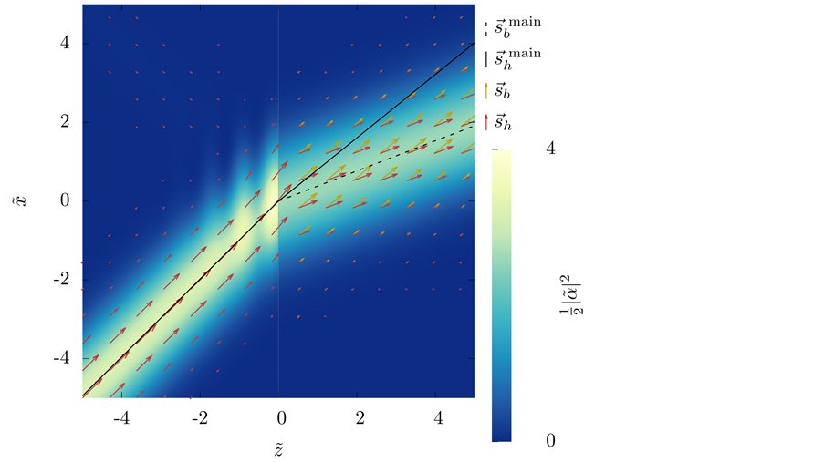
Figure 5. Refraction of the Gaussian beam from vacuum towards the SRR for 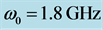 and
and . We plot a measure of the energy density (in the color map), the
  and
and  fields (as vector fields), and the direction of the
  and
and  for the main mode of the beam (as lines).
Figure 6. Refraction of the Gaussian beam from vacuum towards the SRR for  and
and . We plot a measure of the energy density (in the color map), the
  and
and  fields (as vector fields), and the direction of the
  and
and  for the main mode of the beam (as lines).
direction of . But actually this is not the case, and we wish to quantify and elaborate briefly on this.
Let us define  and
and . An important question is, taken this as intensities, how would the beam profile vary from the one obtained with the mean energy density
 ? It should be clear that the quotient
  is exactly 1 on vacuum; on the other side, within the metamaterial we calculated it numerically for the same setups presented in Figure 2, Figures 4-6; it is practically constant, with a slow variation in the
  direction. For example, for the SRR and parameter values as in Figure 6, this ratio is about 1.2. The slow spatial variation in this proportion can be understood in terms of Equation (49), which allows us to write
 (50)
(50)
Written in this way, we can recognize the term  as the square cosine of the angle formed between
  and the z axis. As we observed in point 6b of the list above, this directions do not seem to vary along space. All this tells us that the beam profiles (the “shapes”) predicted by
  and
and  are essentially the same, that they only vary in the prediction of the intensity of the transmitted beam.
On the other hand, note, from Equation (35) that the essential difference between  and
and  (or
(or , in view of the former conclusion) is the magnitude of the gradient of the phase of the electric field
  (which is clearly not constant). In Figure 7 we can see the quotient
 . This is essentially the magnitude of the gradient of phase, and, as it can be seen, except in the interference zone, it seems “constant”. The quotes here are because the value of that constant is one in the vacuum side and a different one on the metamaterial side.
The numerical analysis of these two quantities  and
and  show two important things: first, that the profile given by
 ,
,  and
and  are essentially the same (and thus there is no bias with respect to this two fields in the choice of plotting
 ); and second, that there is a difference with respect to the predictions of the intensities of the transmitted beams, which manifest in the abrupt change of
  when passing from vacuum to the metamaterial. This last observation is expected, since, for the polarization we are analyzing,
  is continuous, while
  is not. The effect of this discontinuity is―at least for the cases we analyze―desirable from the point of view of experience, because, as Figure 8 and Figure 9 show, the profiles of
  no longer have a more intense transmitted beam than the incident one, as it does happen in the corresponding Figure 2 and Figure 4.
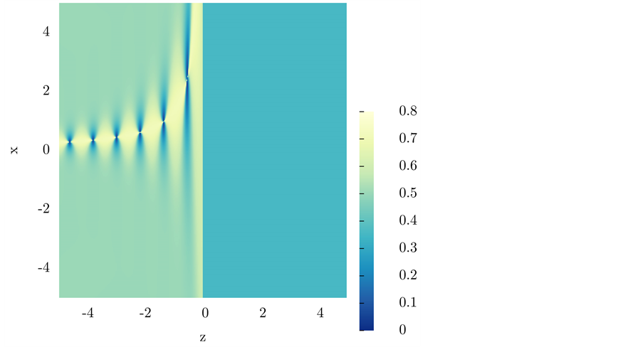
Figure 7. Proportion between  and
and  for the SRR at 2 GHz and an incidence angle of
 . This plot corresponds to the same parameters as Figure 5.
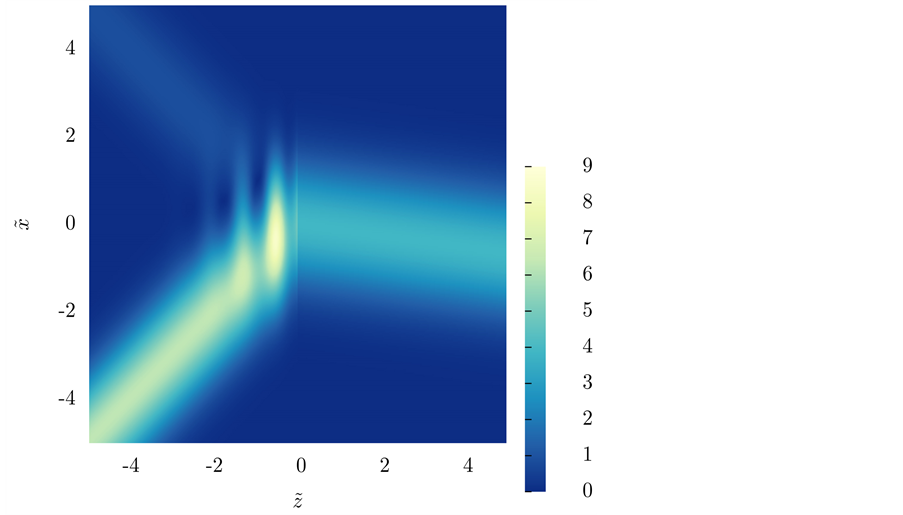
Figure 8. Magnitude of  for the same parameters of Figure 2.
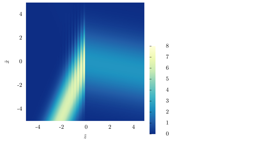
Figure 9. Magnitude of  for the same parameters of Figure 4.
The discussion of the intensity predictions of the two choices of the Poynting vector also leads to an intere- sting question: Since we define intensity as proportional to the energy density, one could ask if there exists a device capable of responding to this quantity. Consider an idealized “intensity detector” consisting of a small plane screen, whose detection result is the integration of the intensity over such surface. Center this detector in a point along the axis of the Gaussian beam. First, put the screen aligned with the axis and take a measure with this device. Afterwards, put the screen in the orthogonal position (remember this is a 2D beam) and take a second measure. Since in the first case the axis coincides with the line of maxima of intensity, the measure is necessarily greater than in the second. But our experience with detectors tells us this is not the case; in fact, it is exactly opposite. This is important because, since  and
and  produce the same intensity profiles, one could think that there is no practical difference if the flux comes from one or the other, because it is the profile what we measure. But if we accept that the detector in some way reacts to the energy flux (as a vector quantity) through the surface integral of its projection over the screen's normal, the maximum value would be obtained, with
 , when the screen is orthogonal to the axis, while for
  it would be obtained in different directions, as it can be seen in Figure 2, Figures 4-6. With this assumption, to measure the intensity at a given point one has to either know the direction of flow a priori, or rotate the detector (with normal
 ) in all possible directions, obtaining a measure of
  for each direction; when this quantity is the greatest of all (
 , with
  parallel to
 ), one gets the intensity and the direction of the energy flow in that point.
It is also important to stress that the results we show here make evident that in general the ray directions in the formalism of geometrical optics and the notion of a ray as an idealized narrow beam (characterized by its intensity) are not equivalent.
6. Conclusions
We discussed the choice between two possible expressions for the Poynting vector: 1)  and 2)
 , in order to discriminate which of them truly represents the direction of energy flow within anisotropic media. We construct a 2D monochromatic beam and calculate how this beam refracts at an interface between vacuum and an uniaxial anisotropic metamaterial, at frequency bands in which dissipation is negligible and with optical parameters unrestricted with respect to sign. The results obtained make us conclude that:
1) For any monochromatic 2D field and in any medium (even absorbing ones) there is a “ray” formalism which extends the eikonal formalism. The directions of those “rays” are given, in s polarization, by , and in p polarization by
 .
.
2) The directions of the rays, defined in this work as idealized narrow beams, coincide within the simulations presented here with the Poynting vector if we define it as  rather than
 . Thus:
a) The “ray” formalism described in conclusion 1 (and therefore the eikonal formalism) is not equivalent to the “intuitive” notion of light ray given by idealized narrow beams.
b) Following the geometrical criterion proposed here, the field  is more suitable as a definition of the energy flux compared to
 .
.
c) The definition of light ray as an idealized narrow beam and the results obtained here allow us to associate the light rays with the field lines of the  vector.
Acknowledgements
We would like to thank Vadim A. Markel for stimulating discussion at the early stages of this project; Augusto García-Valenzuela and Roberto Alexander-Katz for their comments and the full review of the paper; and to Víctor Romero-Rochín for very interesting discussions related to topics about energy conservation. One of us (CP-L) must acknowledge that the work presented here was supported by a graduate scholarship granted by Consejo Nacional de Ciencia y Tecnología (México).
Cite this paper
Carlos Prieto-López,Rubén G. Barrera, (2016) Electromagnetic-Energy Flow in Anisotropic Metamaterials: The Proper Choice of Poynting’s Vector. Journal of Modern Physics,07,1519-1539. doi: 10.4236/jmp.2016.712139
References
- 1. Chen, H., Zhang, J., Bai, Y., Luo, Y., Ran, L. and Jiang, Q. (2006) Optics Express, 14, 12944-12949.
http://dx.doi.org/10.1364/OE.14.012944 - 2. Papadakis, G.T., Yeh, P. and Atwater, H.A. (2014) Physical Review B, 91, Article ID: 155406.
- 3. Prieto-López, C. and Barrera, R.G. (2012) Physica Status Solidi (b), 249, 1110-1118.
http://dx.doi.org/10.1002/pssb.201100747 - 4. Malacara-Hernández, D. and Malacara-Hernández, Z. (2003) Handbook of Optical Design. 2nd Edition, CRC Press, Boca Raton.
http://dx.doi.org/10.1201/9780203912942 - 5. Kline, M. and Kay, I.W. (1965) Electromagnetic Theory and Geometrical Optics. Interscience Publishers, Hoboken.
- 6. Alonso, M.A. (2010) Phase-Space Optics: Fundamentals and Applications. McGraw-Hill Professional, New York.
- 7. Costa, J.T., Silveirinha, M.G. and Alù, A. (2011) Physical Review B, 83, Article ID: 165120.
http://dx.doi.org/10.1103/physrevb.83.165120 - 8. Boardman, A.D. and Marinov, K. (2006) Physical Review B, 73, Article ID: 165110.
http://dx.doi.org/10.1103/physrevb.73.165110 - 9. Ruppin, R. (2002) Physics Letters A, 299, 309-312.
http://dx.doi.org/10.1016/S0375-9601(01)00838-6 - 10. Cui, T.J. and Kong, J.A. (2004) Physical Review B, 70, Article ID: 205106.
http://dx.doi.org/10.1103/physrevb.70.205106 - 11. Ziolowski, R.W. and Heyman, E. (2001) Physical Review E, 64, Article ID: 056625.
- 12. Tretyakov, S.A. (2005) Physics Letters A, 343, 231-237.
http://dx.doi.org/10.1016/j.physleta.2005.06.023 - 13. Simovski, C.R. and Tretyakov, S.A. (2007) Physical Review B, 75, Article ID: 195111.
http://dx.doi.org/10.1103/physrevb.75.195111 - 14. Richter, F., Henneberger, K. and Florian, M. (2010) Physical Review B, 82, Article ID: 037103.
http://dx.doi.org/10.1103/physrevb.82.037103 - 15. Kinsler, P., Favaro, A. and McCall, M.W. (2009) European Journal of Physics, 30, 983-993.
http://dx.doi.org/10.1088/0143-0807/30/5/007 - 16. Obukhov, Y.N. and Hehl, F.W. (2003) Physics Letters A, 311, 277-284.
http://dx.doi.org/10.1016/S0375-9601(03)00503-6 - 17. Richter, F., Florian, M. and Henneberger, K. (2008) Europhysics Letters, 81, 67005-67009.
http://dx.doi.org/10.1209/0295-5075/81/67005 - 18. Silveirinha, M.G. (2010) Physical Review B, 82, Article ID: 037104.
http://dx.doi.org/10.1103/physrevb.82.037104 - 19. Silveirinha, M.G. (2009) Physical Review B, 80, Article ID: 235120.
http://dx.doi.org/10.1103/physrevb.80.235120 - 20. Mansuripur, M. (2011) Optics Communications, 284, 594-602.
http://dx.doi.org/10.1016/j.optcom.2010.08.079 - 21. Markel, V.A. (2009) Optics Express, 17, 7325-7327.
http://dx.doi.org/10.1364/OE.17.007325 - 22. Marqués, R. (2009) Optics Express, 17, 7322-7324.
http://dx.doi.org/10.1364/OE.17.007322 - 23. Markel, V.A. (2008) Optics Express, 16, 19152-19168.
http://dx.doi.org/10.1364/OE.16.019152 - 24. Mischenko, M.I. (2014) Journal of Quantitative Spectroscopy & Radiative Transfe, 146, 4-33.
http://dx.doi.org/10.1016/j.jqsrt.2014.02.033 - 25. Pfeifer, R.N.C. and Nieminen, N.R. (2007) Reviews of Modern Physics, 79, 1197-1216.
http://dx.doi.org/10.1103/RevModPhys.79.1197 - 26. Minkowsky, H. (1910) Mathematische Annalen, 68, 472-525.
http://dx.doi.org/10.1007/BF01455871 - 27. Abraham, M. (1909) Annalen der Physik, 322, 891-921.
http://dx.doi.org/10.1007/bf03018208 - 28. Ginzburg, V.L. (1973) Soviet Physics Uspekhi, 16, 434.
http://dx.doi.org/10.1070/PU1973v016n03ABEH005193 - 29. Roche, J.J. (2000) American Journal of Physics, 68, 438-449.
http://dx.doi.org/10.1119/1.19459 - 30. Nelson, D.F. (1996) Physical Review Letters, 76, 4713-4716.
http://dx.doi.org/10.1103/PhysRevLett.76.4713 - 31. Campos, I. and Jiménez, J.L. (1992) European Journal of Physics, 13, 117-121.
http://dx.doi.org/10.1088/0143-0807/13/3/003 - 32. Furry, W.H. (1969) American Journal of Physics, 37, 621-636.
http://dx.doi.org/10.1119/1.1975729 - 33. Mansuripur, M. and Zakharian, A.R. (2009) Physical Review E, 79, Article ID: 026608.
http://dx.doi.org/10.1103/physreve.79.026608 - 34. Feynman, R.P., Leighton, R.B. and Sands, M. (1964) The Feynman Lectures on Physics. Volume 2, Addison-Wesley, Upper Saddle River.
- 35. Barrera, R.G., Mochán, W.L., García-Valenzuela, A. and Gutiérrez-Reyes, E. (2010) Physica B Condensed Matter, 405, 2920-2924.
http://dx.doi.org/10.1016/j.physb.2010.01.004 - 36. Henrotte, F. and Hameyer, K. (2006) IEEE Transactions on Magnetics, 42, 903-906.
http://dx.doi.org/10.1109/TMAG.2006.871441 - 37. Gough, W. (1982) European Journal of Physics, 3, 83-87.
http://dx.doi.org/10.1088/0143-0807/3/2/005 - 38. Romer, R.H. (1982) American Journal of Physics, 50, 1166-1168.
http://dx.doi.org/10.1119/1.12903 - 39. Peters, P.C. (1982) American Journal of Physics, 50, 1165.
http://dx.doi.org/10.1119/1.13024 - 40. Lai, C.S. (1981) American Journal of Physics, 49, 841-843.
http://dx.doi.org/10.1119/1.12719 - 41. Slepian, J. (1942) Journal of Applied Physics, 13, 512-518.
http://dx.doi.org/10.1063/1.1714903 - 42. Landau, L.D. and Lifshitz, E.M. (1984) Electrodynamics of Continuous Media. Pergamon Press, Oxford.
- 43. Jackson, J.D. (1998) Classical Electrodynamics. 3rd Edition, John Wiley & Sons Inc., Hoboken.
- 44. Brillouin, L. (1960) Wave Propagation and Group Velocity. Academic Press, New York.
NOTES

1http://www.fisica.unam.mx/personales/rbarrera/gaussian-beam.