Journal of Modern Physics
Vol.3 No.9A(2012), Article ID:23092,7 pages DOI:10.4236/jmp.2012.329157
Confidence Level Estimator of Cosmological Parameters
Physics Department, University of Milano Bicocca, Milano, Italy
Email: giorgio.sironi@unimib.it
Received June 21, 2012; revised July 24, 2012; accepted July 31, 2012
Keywords: Cosmological Models; Cosmological Parameters
ABSTRACT
Cosmological Models frequently suggest the existence of physical, quantities, e.g. dark energy, we cannot yet observe and measure directly. Their values are obtained indirectly setting them equal to values and accuracy of the associated model parameters which best fit model and observation. Apparently results are so accurate that some researchers speak of precision cosmology. The accuracy attributed to these indirect values of the physical quantities however does not include the uncertainty of the model used to get them. We suggest a Confidence Level Estimator to be attached to these indirect measurements and apply it to current cosmological models.
1. Introduction
Models of physical systems, including Cosmological Models, contain a number of free parameters associated to an equal number of measurable, independent, physical quantities (“observable” in the following) which characterize the system. Comparing measured values of the observables and allowed values of the parameters one can test a model, i.e. validate, improve or falsify it [1].
When a model introduces new parameters associated to observables previously ignored or never observed, searching and measuring the new observables is mandatory.
Some observables can be measured directly (e.g. galaxy redshift) or through a serie of definite, model independent, intermediate steps (e.g. object distance by parrallax). Let’s call them direct measurements.
Other observables (e.g. Dark Energy density we will discuss in the following), cannot yet be measured directly. We get their values looking to secondary observables linked in a way we presume we know to the primary observable we are interested in. Let’s call them indirect measurements. The reliability of indirect measurements depends therefore on the accuracy of the link model, preferably an “ad hoc” model, with a reduced number of parameters, especially made for the particular observable we intend to measure, but in some cases it is the Model itself we want to test.
Present days cosmological models give a fair description of the birth and evolution of the Universe using six free parameters. Mostly of the associated observables are however measured indirectly.
In the following we discuss first the error bars associated to direct and indirect measurements of observables, then introduce an estimator (Confidence Level Estimator) to quantify the confidence we can attach to indirect measurements. We then briefly review present day most common Cosmological Models and apply to their parameters and observables our Confidence Level Estimator.
2. Observables: Expected and Measured Values
Results of independent direct measurements of an observable  give a serie
  of data which, analyzed by classical statistical methods (see for instance [2]) give mean value
  and standard deviation
  of
of . We call them measured values of
 .
.
When  must be measured indirectly we collect by direct observation or from data in literature values of secondary observables associated to
 , specify the model of the link between
  and those secondaries and attach to X the value of the associated model parameter
  which best fits model and values of the secondary observables. When considering Cosmological Models the best fitting procedure is usually made by Montecarlo methods: one repeats the evaluation of
  with a random choice of the Model parameters and gets a distribution of
  values around a value
 , which optimizes the fit. We then set
  and attach to it a dispersion
  equal to the width of the distribution of the
  values around
  which encompasses 68% of the values. We call them expected values. However
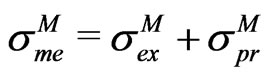
  does not include information on how reliable is the model of the link between primary and secondary observables therefore is different from
 . If we are extremely confident in the model we can set
 . If not we must write
  where
where  is a sort of systematic error which accounts for Model uncertainty.
2.1. Single Parameter Model
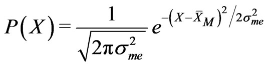
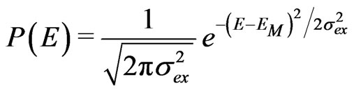
Let’s begin with a Model with just one parameter M. We call  the distribution, around
 , of the directly measured values X of the observable and
  the distribution, around
 , of the values attributed to parameter M. Most often
  and
and  are gaussian
 (1)
(1)
 (2)
(2)
when

 and
and  overlap marginally and the Model does not describe properly the physical system associated to the observable.
When

 and
and  begin to overlap and the Model may be more descriptive of the physical system.
For models and priors1 not too far from the real world
 (3)
(3)
and differences between  and
and  can be entirely attributed to differences between
  and
and , so we can write
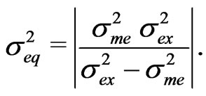
Evaluating  is far from obvious. We introduce instead
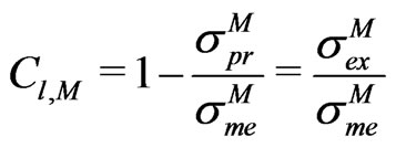 (4)
(4)
and call it Confidence Level Estimator of the observable associated to M.
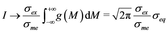
For direct measurements  therefore
  always. For secondary measurements
  because
 .
.  suggests that Model, priors and observation do not conflict therefore the Model offer a convenient way for improving
 . When
  Model and priors cannot be used for improving
  and very probably do not offer a completely correct description of the real world.
More formal derivations of  are possible. In Appendix A we propose a derivation
  from the Bayes Theorem.
2.2. Multiparameter Model
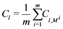
For a model with  independent parameters we can write:
 (5)
(5)
as a collective estimator of the set of Model parameters. It is the average of the , (see Equation (4)), associated to the Model
  parameters. Its value is also indicative of Model and priors qualities.
Small values of Confidence Levels obtained by Equations (4) and (5) cannot be used to falsify the Model used to get them. Falsification in fact occurs only when the two probability distributions  and
and  do not overlap at all. When this is the case condition (3) and Equations (4) and (5) do not hold anymore.
3. Cosmological Models
The almost serendipitous discovery of the Cosmic Microwave Background in 1964 [3]: 1) marked the end of a famous revised version of the Steady State Model, proposed in 1948 by Bondi, Gold and Hoyle [4,5], in spite of its capability of preserving fundamental constants of physics and avoiding singularities during the Universe expansion; 2) boosted the class of the Big Bang Models (e.g. [6]). Difficulties of this class of models, like the initial singularity and the problem of “causal connections”, were soon solved by the inclusion of the Inflation theory (see for instance [7]) with the additional bonus of gaining the possibility of estimating the spectrum of the primordial fluctuations, necessary to explain the birth of the matter condensations which characterize the present day Universe (for a review see for instance [8]); 3) triggered new cosmological observation of the CMB which, in about thirty years, confirmed that the CMB has: a) planckian spectrum ([9-11] and references therein); b) a small degree of anisotropy with a characteristic angular power spectrum ([12-14] and references therein); c) an even smaller degree of linear polarization ([15-18] and references therein).
So gradually the Standard Big Bang Model ([6]) emerged, whose more important parameters were: Hubble constant , Universe matter density
  (in units of critical density
 ) and primordial Helium Hydrogen ratio.
In the same years other no-CMB based cosmological observations went on. They: 1) provided large samples of high redshift Supernovae (see for instance the Supernova Cosmological Project [19]), used to obtain better estimates of matter density and upper limit to the value of the cosmological constant); 2) showed the existence of dark matter at various astrophysical sites (for a review see for instance [20]); 3) detected Baryon Acoustic Oscillations (BAO) in the ordinary matter distribution with an angular power spectrum similar to the angular power spectrum of the CMB ([21] and references therein); 4) got the distances of objects at very large Z using new standard candles (SNIa and GRB) (e.g. [22,23] and references therein). Not to mention the results of numerical experiments (Nbody simulations) on the formation and evolution of matter condensations (e.g. [24]).
The whole set of CMB and no-CMB observations suggests that: 1) the geometry of the Universe is euclidean (flat) or very close to it [25]; 2) recombination of nuclei and electrons at  was followed by partial reionization of the matter when stable matter condensations formed (e.g. [26] and references therein); 3) after decelerating, the Universe is now going through re-acceleration (e.g. [27]).
To account for these effects new cosmological parameters were introduced: 1) ,
,  and
and , the abundances (in unit of critical density
![]() ) of barionic matter, dark matter and dark energy; 2)
) of barionic matter, dark matter and dark energy; 2) , the optical thickness of the Universe at reionization; 3)
  and
and , the amplitude and spectral index of the fluctuations; 4)
  an indicator of the galactic matter distribution. Adding them to the Standard Big Bang Model the Concordance or
  Model emerged [28,29]. It is characterized by six independent parameters plus a number of derived parameters, combinations of the independent ones. Usually
 ,
,  ,
,  ,
,  ,
,  and
and , are assumed as free parameters. Among the derived parameters are age of the Universe
 , critical density
  of matter-energy, Dark Energy density,
  (in unit of
 ), reionization red shift
  and
and .
.
Usually observation gives combinations of the observables associated to the above parameters. To disentangle them it is common practice to fit the Concordance Model to the full set of CMB and no-CMB data and extract the parameters values which best fit observation. Calculations are made by Montecarlo methods [30] using Markov chains to implement the stochastic procedure with the addition of priors which constrain the variability of the model parameters. Common choices are  (perfectly euclidean Universe) and
 . By this method one gets the expectation values of the model parameters and their dispersion, (set equal to the width of the distribution of the calculated values E which encompasses 68% of the values) and attach them to the associated observables.
The procedure, now well established, is usually repeated whenever new data are added to the preexisting data base of observations. Very probably it will be repeated when the new CMB data presently being collected by the Planck mission will be released [31]. Table 1 and Table 2 show expectation values  and dispersion
  of free and derived parameters M of the Concordance Model in literature [18,32,34]. Because different authors use different combinations of parameters and/or different units of measure, for uniformity of presentation in Tables 1 and 2, when necessary, the listed quantities have been obtained transforming the data in literature (preserving the published value of the combination).
In the same table are listed, when available, mean value  and standard deviation
  of direct measurements X of the observable associated to M.
It appears that for five, out of six, free parameters of the Concordance Model direct measurements of the associated observable are poor or not yet available. In particular observation gives only large intervals inside which measured values of the density of Dark Matter and Dark Energy can lay. These intervals coincide with the variability range of the parameters used in Monte Carlo studies of the Concordance Model [18]. The only exception is the Hubble constant for which accurate measurements now exist [33].
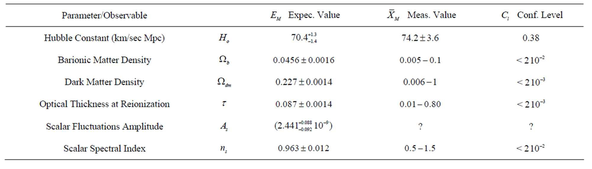
Table 1. -Concordance Model: expectation values, measured values and confidence level of model parameters (from [34,18] see text).

Table 2.  -Concordance Model: expectation values of derived parameters (from [18,34] see text).
The above values of  are so small that today is common practice to speak of Precision Cosmology (e.g. [35,36]) and very probably they will be further reduced when the Planck results will appear. A caveat is however necessary: generally
  and in some cases
 . So when model assumptions fail,
  might be optimistic and the stated precision of inference might understate the actual uncertainty of the observable.
4. Discussion
Analysis of cosmological observation and deduction of cosmological parameters in literature not always explicitly refers to Bayesian statistics so the language used is not necessarily the one which would be used by a Bayesian statistician (see [37] and references therein) Bayesian statistics however can provide useful hints at least about:
1) Dispersion of the priors (see for instance [38] and references therein). In its more common implementations the Concordance Model sets the very stringent limits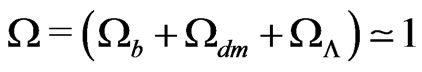 . Assuming a Bayesian point of view there is therefore a risk that the priors on
 ,
,  ,
,  and
and  are underdispersed, undermining the validity the analysis results. Therefore these limits probably have to be relaxed.
2) Robustness of the results (see for instance [39] and references therein). The results so far published do not show evidence of oscillations of the values of the Concordance Model parameters around their expectation values, confirming that from a Bayesian point of view these results are robust.
But our Confidence Level Estimators hold also outside the borders of Bayesian Statistics. Expression (14) has been in fact obtained also on empirical basis (see Equation (4)).
So we will use our Estimators to evaluate the weight we can attach to observables and cosmological parameters provided by the Concordance Model, no matter if the procedures the authors ([18,32,34] and references therein) used to get them are fully Bayesian or not.
The last Column of Table 1 shows the Confidence Levels of the Concordance Model free parameters, calculated by Equation (4) and approximation (3). For the whole Model, Equation (5) gives
They do not falsify the Concordance Model (the distributions of the expected values of all the parameters of the Concordance Model are well inside the uncertainty intervals of the measured values).
However, with the exception of the Hubble constant, the differences  of the parameters are so large that
  (see Section 2) and the role played by Model and priors can’t be neglected. So we cannot assume the expectation values of some parameters of the Concordance Model as representative of the values of the associated observables, for instance when studying astrophysical situations where dark matter, dark energy, if present, are important.
This leaves open the possibility of considering other Models of the Universe different from the Concordance Model which is based on the strong double condition . We can for instance keep
  and relax the condition
 , assuming a different recipe of the Universe composition, e.g. without or with a reduced quantity of Dark Energy, an exigency remarked also very recently (see for instance the comments by [40]). In fact: 1) no direct evidence for the existence of Dark Energy has been so far obtained; 2)in literature there are models which show the possibilities of producing effects similar to those attributed to the presence of Dark Energy, through inhomogeneities of the matter distribution (e.g. [41]). The work on these Models is still in progress. We cannot yet apply to them the same procedure used with the Concordance Model and extract expectation values for their parameters. Comparison of their Confidence Levels with the Confidence Levels of Table 1 will probably become possible in the near future.
Meanwhile, it is necessary: 1) to improve direct measurements of all the observables associated to the Concordance Model parameters, aiming at  and
and  for all the parameters
 , and/or 2) to get independent evidence of existence and weight of
 , the Dark Energy density.
The above conclusions remain also if one adds to the set of preexisting data results of new indirect evaluations of the Cosmological Parameters more recently published (e.g. [34,42]). Probably they will not change until new direct measurements or indirect measurements based on other independent models will appear.
5. Conclusions
The use of Montecarlo methods and Bayesian Statistics to analyze the enormous quantity of data of cosmological interest which are continously poured by ground and space observations is almost unavoidable. However Montecarlo and Bayesian Methods are based on assumption (models and priors) whose statistical weight should be added, but rarely is added, to the the quoted accuracies of the parameter expectation values.
Researchers who currently use these methods are aware of that and warning has been already put forward (e.g. [36,43]). Unfortunately general public and professionals not involved in cosmological observations may be unaware of it, misinterpret the results of model simulations and attribute weights above their real values to models. Forgetting it may stop or reduce support to studies of other models not yet excluded by observation.
This situation is common to other fields of pure and applied research (e.g. unification of fundamental forces, string theories, elementary particle models, models of climate evolution and so on). The Confidence Level Estimator we propose can be used to avoid misunderstandings and preserve possibilities of pursuing alternatives lines of research also in these fields.
6. Acknowledgements
We acknowledge the support of MIUR (Italian Ministry of University and Research), CNR (Italian National Council of Research), PNRA (Italian Program for Antarctic Research) and (Italian Space Agency) to studies and observations of the CMB properties.
REFERENCES
- K. Popper, “Conjecture and Refutations: The Growth of Scientific Knowledge,” Taylor and Francis, Abingdon, 1989.
- P. R. Bevington and K. D. Robinson, “Data Reduction and Error Analysis for the Physical Sciences,” McGraw-Hill, London, 1992.
- A. A. Penzias and R. A. Wilson, “A Measurement of Excess Antenna Temperature at 4080 Mc/s,” Astrophysical Journal, Vol. 142, No. 7, 1965, pp. 419-421. doi:10.1086/148307
- H. Bondi and T. Gold, “The Steady State Theory of the Expanding Universe,” Monthly Notices of the Royal Astronomical Society, Vol. 108, No. 2, 1948, pp. 252-270.
- F. Hoyle, “A New Model of the Expanding Universe,” Monthly Notices of the Royal Astronomical Society, Vol. 108, No. 3, 1948, pp. 372-382.
- P. J. E. Peebles, “Principles of Physical Cosmology,” Princeton University Press, Princeton, 1993.
- A. H. Guth, “The Inflationary Universe,” Perseus Book, Reading, 1997.
- R. B. Partridge, “3K: The Cosmic Microwave Background Radiation,” Cambridge University Press, Cambridge, 1995. doi:10.1017/CBO9780511525070
- D. J. Fixsen and J. C. Mather, “The Spectral Results of the Far Infrared Absolute Spectrophotometer on COBE,” Astrophysical Journal, Vol. 581, No. 12, 2002, pp. 817- 822. doi:10.1086/344402
- G. F. Smoot, et al., “Low Frequency Measurements of the Cosmic Bacground Radiation Spectrum,” The Astrophysical Journal Letters, Vol. 291, No. 4, 1985, pp. L23-L27. doi:10.1086/184451
- M. Zannoni, et al., “TRIS I: Absolute Measurements of the Sky Brightness Temperature at 0.6, 0.82 and 2.5 GHz,” Astrophysical Journal, Vol. 688, No. 11, 2008, pp. 12-23. doi:10.1086/592133
- C. L. Bennett, et al., “Four-Year COBE DMR Cosmic Microwave Background Observations: Maps and Basic Results,” Astrophysical Journal, Vol. 464, No. 6, 1996, pp. L1-L4. doi:10.1086/310075
- D. Larson, et al., “Seven-Years Wilkinson Microwave Anisotropy Probe (WMAP) Observations: Power Spectra and WMAP-Derived Parameters,” The Astrophysical Journal Supplement, Vol. 192, No. 16, 2011, pp. 1-19.
- R. B. Friedman, et al., “Small Angular Scale Measurements of the Cosmic Microwave Background Temperature Power Spectrum from QUaD,” Astrophysical Journal, Vol. 700, No. 8, 2009, pp. L187-L191. doi:10.1088/0004-637X/700/2/L187
- A. Kogut, et al., “Five-Year Wilkinson Microwave Anisotropy Probe (WMAP) Observations: Temperature-Polarization Correlatioin,” The Astrophysical Journal Supplement, Vol. 148, No. 9, 2003, pp. 161-173. doi:10.1086/377219
- F. Piacentini, et al., “A Measurement of the PolarizationTemperature Angular Cross-Power Spectrum of the Cosmic Microwave Background from the 2003 Flight of BOOMERANG,” Astrophysical Journal, Vol. 647, No. 8, 2006, pp. 833-839. doi:10.1086/505557
- G. Polenta, et al., “The BRAIN CMB Polarization Experiment,” New Astronomy Reviews, Vol. 51, No. 3, 2007, pp. 256-259. doi:10.1016/j.newar.2006.11.065
- M. L. Brown, et al., “Improved Measurements of the Temperature and Polarization of the Cosmic Microwave Background from QUaD,” Astrophysical Journal, Vol. 705, No. 4, 2009, pp. 978-999. doi:10.1088/0004-637X/705/1/978
- S. Perlmutter, et al., “Measurements of Omega and Lambda from 42 High Redshift Supernovae,” Astrophysical Journal, Vol. 517, No. 6, 1999, pp. 565-586. doi:10.1086/307221
- G. Bertone, D. Hooper and J. Silk, “Particle Dark Matter: Evidence, Candidates and Constraints,” Physics Reports, Vol. 405, No. 1, 2005, pp. 279-390. doi:10.1016/j.physrep.2004.08.031
- W. J. Percival, et al., “Baryon Acoustic Oscillations in the Sloan Digital Sky Survey Data Release 7 Galaxy Sample,” Monthly Notices of the Royal Astronomical Society, Vol. 401, No. 2, 2010, pp. 2148-2168. doi:10.1111/j.1365-2966.2009.15812.x
- N. Panagia, “High Redshift Supernovare: Cosmological Implications,” Nuovo Cimento B, Vol. 120, No. 6, 2005, pp. 667-680.
- G. Ghirlanda, G. Ghisellini and C. Firmani, “Gamma Ray Bursts as Standard Candles to Constrain the Cosmological Parameters,” New Jersey Postal History Society, Vol. 8, No. 7, 2006, pp. 123-124.
- M. Macció, et al., “Coupled Dark Energy: Constraints from N-Body Simulations,” Physical Review D, Vol. 69, No. 12, 2004, pp. 123516-123540. doi:10.1103/PhysRevD.69.123516
- P. de Bernardis, et al., “Multiple Peaks in the Angular Power Spectrum of the Cosmic Microwave Background Significance and Consequences for Cosmology,” Astrophysical Journal, Vol. 564, No. 1, 2002, pp. 559-666. doi:10.1086/324298
- P. Valageas and J. Silk, “The Reheating an Reionization History of the Universe,” Astronomy & Astrophysics, Vol. 347, No. 7, 1999, p. 20.
- A. G. Riess, et al., “Observational Evidence from Supernovae for an Accelerating Universe and a Cosmological Constant,” The Astronomical Journal, Vol. 116, No. 9, 1998, pp. 1009-1038.
- J. P. Ostriker and P. J. Steihardt, “Cosmic Concordance,” 1995, arXiv:astro-ph/9505066v1.
- M. Kowalski, et al., “Improved Cosmological Constraints from New, Old and Combined Supernova Data Sets,” Astrophysical Journal, Vol. 686, No. 10, 2008, pp. 749-778. doi:10.1086/589937
- D. P. Landau and K. Binder, “A Guide to Monte-Carlo Simulations in Statistical Physics,” Cambridge University Press, Cambridge, 2009. doi:10.1017/CBO9780511994944
- Planck Science Team, “Planck Science Team Home,” 2012. http://www.rssd.esa.int/index?project=Planck
- E. Komatsu, et al., “Five-Year Wilkinson Microwave Anisotropy Probe Observations: Cosmological Interpretation,” The Astrophysical Journal Supplement, Vol. 180, No. 2, 2009, pp. 330-376. doi:10.1017/CBO9780511994944
- A.G. Riess et al., “A Redetermination of the Hubble Constant with the Hubble Space Telescope from a Differential Distance Ladder,” Astrophysical Journal, Vol. 699, No. 7, 2009, pp. 539-563. doi:10.1088/0004-637X/699/1/539
- E. Komatsu, et al., “Seven-Year Wilkinson Microwave Anisotropt Probe (WMAP) Observations: Power Spectra and WMAP-Derived Parameters,” The Astrophysical Journal Supplement, Vol. 192, No. 18, 2011, pp. 1-47.
- J. R. Primack, “Precision Cosmology,” New Astronomy Reviews, Vol. 49, No. 5, 2005, pp. 25-34
- S. L. Bridle, O. Lahav and J. P. Ostriker, “Precision Cosmology? Not Just Yet ...,” Science, Vol. 299, No. 3, 2003, pp. 1532-1533. doi:10.1126/science.1082158
- J. Joyce, “Bayes Theorem,” In: E. N. Zalta, Ed., The Stanford Encyclopedia of Philosophy, The Metaphysics Research Lab, Stanford, 2008. http://plato.stanford.edu/entries/bayes-theorem/
- J. K. Ghosh, M. Delampady and T. Samanta, “An Introduction to Bayesian Analysis,” Springer, New York, 2006.
- J. O. Berger, et al., “Bayesian Robustness,” IMS, Hayward, 1996.
- A. Cho, “A Recipe for Cosmos,” Science, Vol. 330, No. 12, 2010, pp. 1615-1616. doi:10.1126/science.330.6011.1615
- L. Amendola, R. Gannouji, D. Polarski and S. Tsyikawa, “Condition for the Cosmological Viability of f(R) Dark Energy Models,” Physical Review D, Vol. 75, No. 8, 2007, pp. 83504-83560. doi:10.1103/PhysRevD.75.083504
- J. Dunkley, et al., “The Atacama Cosmology Telescope Cosmological Parameyters from the 2008 Power Spectrum,” Astrophysical Journal, Vol. 739, No. 9, 2011, pp. 52-72. doi:10.1088/0004-637X/739/1/52
- R. G. Vishwakarma and J. V. Narlikar, “A Critique of Supernova Data Analysis in Cosmology,” Research in Astronomy and Astrophysics, Vol. 10, No. 1, 2010, pp. 1195-1198.
- R. Swinburne, “Introduction to Bayes’s Theorem,” In: R. Swinburne, Ed., Bayes’s Theorem, Oxford University Press, Oxford, 2002, pp. 1-55.
- S. J. Press, “Bayesian Statistics,” Wiley, New York, 1989.
- AA.VV., “Bayes Theorem,” In: R. K. Bock, K. Bos, S. Brandt, J. Myrheim and M. Regler, Eds., Formulae and Methods in Experimental Data Evaluation, EPS-CERN, Geneva, 1984, p. 7.
Appendix A: Derivation of Cl,M from the Bayes Theorem
Let’s assume (see Section 2.1):
1)  set of “old” or preexisting, model independent, measurements of an observable;
2)  set of “new”, model dependent, measurements of parameter M associated by the model to the observable;
3)  likelihood function of the “old” measurements O;
4)  likelihood function of the “new” measurements N;
5)  posterior conditional probability of O given N;
6)  conditional probability of N, given O, produced by Model and prior.
These quantities are linked by the Bayes Theorem (see for instance [[38,44-46] and references therein) which reads:
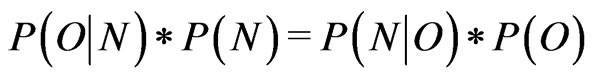 (6)
(6)
We introduce
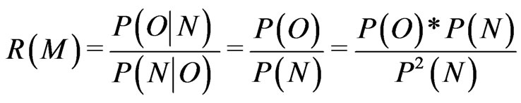 (7)
(7)
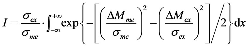
The numerical value of
 (8)
(8)
is proportional to the overlapping of  and
and , a measure of the correlation degree of direct and indirect measurements (when
  and
and  do not overlap
 ). Properly normalized it gives a number
  we can assume as our confidence level indicator of the indirect measurements.
For gaussian distributions of  and
and 
where ,
, .
.
When
 (9)
(9)
 (10)
(10)
and
 (11)
(11)
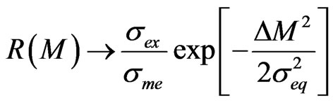
with 
 (12)
(12)
 (13)
(13)
Normalization to the area  covered by
  , gives
 (14)
(14)
identical to our empirical expression (4).
When  and
and  coincide
 . When
 . (
. ( , excluded because
  (see Section 2), would imply models and priors which produce results worse than direct or preexisting measurements).
NOTES
1In different applications meaning and content of prior may be different; here and in the following prior will indicate just the ranges of allowed variability of the Model parameters.