Applied Mathematics
Vol.4 No.6(2013), Article ID:33432,13 pages DOI:10.4236/am.2013.46131
Best Response Games on Regular Graphs
School of Mathematics and Statistics, University of Sheffield, Sheffield, UK
Email: richardsouthwell254@gmail.com, c.cannings@sheffield.ac.uk
Copyright © 2013 Richard Southwell, Chris Cannings. This is an open access article distributed under the Creative Commons Attribution License, which permits unrestricted use, distribution, and reproduction in any medium, provided the original work is properly cited.
Received March 8, 2013; revised April 10, 2013; accepted April 18, 2013
Keywords: Games on Graphs; Cellular Automata; Best Response Games; Social Networks
ABSTRACT
With the growth of the internet it is becoming increasingly important to understand how the behaviour of players is affected by the topology of the network interconnecting them. Many models which involve networks of interacting players have been proposed and best response games are amongst the simplest. In best response games each vertex simultaneously updates to employ the best response to their current surroundings. We concentrate upon trying to understand the dynamics of best response games on regular graphs with many strategies. When more than two strategies are present highly complex dynamics can ensue. We focus upon trying to understand exactly how best response games on regular graphs sample from the space of possible cellular automata. To understand this issue we investigate convex divisions in high dimensional space and we prove that almost every division of k − 1 dimensional space into k convex regions includes a single point where all regions meet. We then find connections between the convex geometry of best response games and the theory of alternating circuits on graphs. Exploiting these unexpected connections allows us to gain an interesting answer to our question of when cellular automata are best response games.
1. Introduction
Game theory is a rich subject which has become more diverse over the years. Early game theory [1] focused on how rational players would behave in strategic conflicts. Concepts like the Nash equilibrium [2] helped theorists to predict final outcomes of games, and this benefited areas like economics. A more recent development is evolutionary game theory [3]. Rather than assuming that players are hyper-rational, evolutionary game theory concerns itself with large populations of players that change their strategies via simple selection mechanisms. Players repeatedly engage in games with other members of the population and the way the populations strategies evolve depends upon the selection mechanism employed.
One way to introduce a spatial aspect into evolutionary games is to imagine the players as vertices within a graph [4,5]. The links represent interactions so vertices play games with their neighbours. The players adapt their strategies over time to try to increase their success against neighbours. Many kinds of update rules have been investigated. These include imitation, where vertices imitate their most successful neighbour, and best response, where vertices update to employ the strategy best suiting their current surroundings. In [6] the authors study a twodimensional cellular automata with update rules based upon games, beautiful patterns emerge.
In previous studies we investigated the dynamics of games on networks where the players update asynchronously [7-10] as they engage in congestion games (where an individual’s payoff decreases with the number of their neighbours using the same strategy). We have also investigated more exotic scenarios, where the network structure itself changes as a result of the strategic interactions between the players/vertices. These type of game based network dynamics can produce remarkably complex structures despite being based upon extremely simple rules, involving reproducing vertices [11-14]. In some of these game based network growth systems, small initial networks can lead to the creation of thousands of different structures which morph and self replicate in complex ways [15,16].
The update mechanism that we concentrate upon in this paper is best response, where vertices update to employ the strategy that maximise their total payoff in a game with each neighbour. The vertices update their strategies myopically and synchronously (i.e., in this paper we focus on systems where all players update their strategies simultaneously, every time step). The strategy a vertex updates to may not be optimal because neighbouring vertices change their strategies at the same time. Work on these kind of systems includes [17] and [18], where it was shown that a two strategy game running upon any graph will eventually reach a fixed point or period two orbit. Two strategy best response games on various graph structures were also studied in [19].
The systems we consider are essentially cellular automata with update rules that are induced by the details of the game. In our consideration of best response games on the circle we will see many of Wolfram’s 256 elementary cellular automata [20] appear. Under these models the states of the vertices on a circle or line graph take values in {0,1}. The states of vertices change with time so that the future state of any cell depends upon the current state of itself and its neigbours. Each systems is specified by a mapping 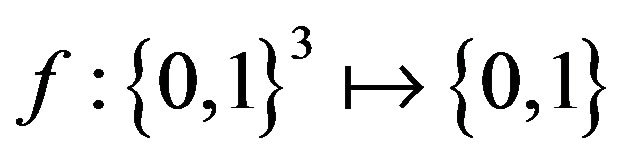 so that
  is the future state of a vertex in state
  with neighbours in states
  and
and  to its left and right. Each system is indexed with a number

We concentrate upon games on the circle because they provide the easiest ways to illustrate our results. Our methods can easily be extended to other graph structures, even non-regular ones.
1.1. Definitions
For a set ![]() let
let  to be the set of size
 ![]() multi sets of elements from
multi sets of elements from ![]() i.e.
i.e.  is the set of all unordered
 ![]() -tuples
-tuples  of members of
![]() , including those
, including those ![]() -tuples containing more than one of the same element. Let us define a regular automata as a quad
-tuples containing more than one of the same element. Let us define a regular automata as a quad , where
  is a regular degree
 ![]() graph,
graph, ![]() is a set of states,
is a set of states,  is an assignment of a state
  to each vertex
  (the initial configuration) and
 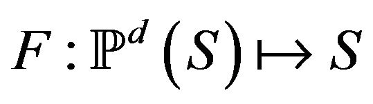 is the update function/rule.
Such a regular automata evolves so that at time step , the future state of a vertex
![]() , at time
, at time , will be
 (1.1)
(1.1)
where
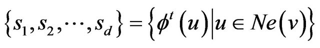 (1.2)
(1.2)
is the set of states of vertices in![]() ’s neighbourhood,
’s neighbourhood,  , at time
 .
.
A game  consists of a set of strategies
  which we label with integers, together with a
  payoff matrix
  such that
  is the payoff that a player receives from employing the
  th strategy against the
  th strategy.
The best response games we consider take place on a degree ![]() regular graph
regular graph . At time
  each vertex
  employs a strategy
 . The total payoff
 (1.3)
(1.3)
of ![]() at time
at time  is the sum of payoffs that
  receives from using its strategy in a game with each neighboring player. At time
  each vertex simultaneously updates its strategy, so that at time
  it will employ the strategy that would have maximised its total payoff, given what its neighbours played at time
 . In other words each player updates to play the best response to its current surroundings.
Best response games on regular graphs are quads
 , which are defined by a regular graph
 , a game
  and an assignment
  of an initial strategy to
  to each vertex of
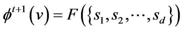
 . A best response game is a regular automata
 with an update function F such that, for every unordered
 ![]() -tuple of strategies
-tuple of strategies
 , we have
  is the strategy in
  that maximises
 (1.4)
(1.4)
We refer to  as the update function induced by the game
 . Note that in rare cases the payoff matrix could be such that two strategies are tied as best responses to a possible local strategy configuration
 . In such a case
  is not properly defined. Such a problem can always be alleviated by an infinitesimal perturbation of the elements in the payoff matrix
 . We always assume our matrix is such that this problem never occurs.
1.2. Examples on the Circle
The circle graph  has vertices
  with
with ![]() is adjacent to
is adjacent to  if and only if
 .
.
Every best response game  on the circle is a regular automata
 , where the strategy
  employed by vertex
 ![]() at time
at time
 will be
 , which is the strategy that maximises the vertices’s total payoff against its neighbours strategies
  and
and
 .
.
The payoff matrix
 (1.5)
(1.5)
is a Hawk-Dove game, where 1 is the passive dove strategy and 2 is the aggressive hawk strategy. Let us consider the best response game , where
  and M is as above. This corresponds to the regular automata
  with update function
 ,
,  and
and
 . We picture how this automata will evolves on a 30 vertex circle from a random strategy configuration, with the space time plot pictured in Figure 1.
A space time plot [20] is a grid where the ![]() axis is the index of the vertex of the circle and the
axis is the index of the vertex of the circle and the ![]() axis (reading downwards) is the time step. Light gray blocks denote employers of strategy 1 whilst dark blocks represent employers of strategy 2. In our game a player adjacent to an employer of dove and employer of hawk gets updated to play the hawk strategy, hence if a block on our space time plot has a dark gray block on its left and a light gray block on its right then the block below it will be dark gray. The system corresponds to Wolfram’s cellular automata number 95, which is well known to have simple dynamics. Every initial configuration evolving quickly to a fixed point or period 2 orbit. This system is an example of a threshold game [17,18].
axis (reading downwards) is the time step. Light gray blocks denote employers of strategy 1 whilst dark blocks represent employers of strategy 2. In our game a player adjacent to an employer of dove and employer of hawk gets updated to play the hawk strategy, hence if a block on our space time plot has a dark gray block on its left and a light gray block on its right then the block below it will be dark gray. The system corresponds to Wolfram’s cellular automata number 95, which is well known to have simple dynamics. Every initial configuration evolving quickly to a fixed point or period 2 orbit. This system is an example of a threshold game [17,18].
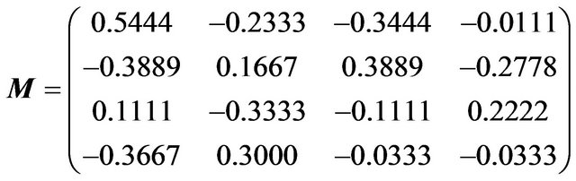
More complicated dynamics occur under the 3 strategy game with payoff matrix
 (1.6)
(1.6)
Figure 2 shows the evolution of the system from a random initial configuration on a 60 vertex circle over 40 time steps. In this case dark gray, white and light gray blocks represent strategies 1, 2 and 3 respectively. The resulting cellular automata can be reduced to Wolfram’s cellular automata number 90 which has been proven to be chaotic [21] when running on an infinite circle.
In this paper we will enumerate all the update functions  that can be induced by 2, 3 or 4 strategy best response games on the circle by consideration of the convex geometry behind best response game. Understanding this convex geometry allows one to understand how the update rules of arbitrary best response games are induced.
1.3. Overview
In Section 2 we discuss some important relationships between best response games and divisions of the simplex into convex regions. By using games on the circle as examples, we describe the relationships with convex divisions, and then present Theorem 2.1, which is our key
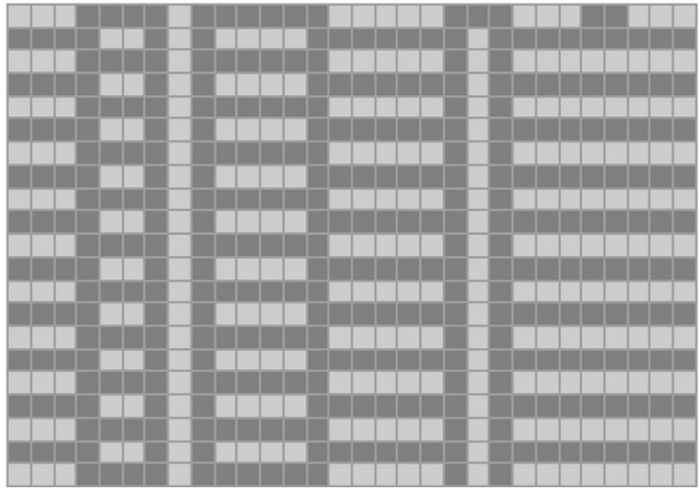
Figure 1. A space time plot showing the evolution of the Hawk-Dove example game on the circle.
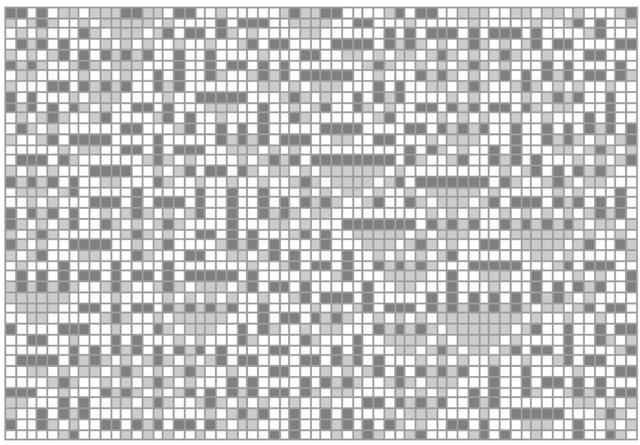
Figure 2. A space time plot showing the evolution of the three strategy game described by the payoff matrix in Equation (1.6).
theoretical result.
In Section 3 we discuss how our theory of convex divisions can be used to find all the different best response games on the circle which have two or three strategies. We also describe the dynamics of the different two strategy games on the circle, and point out relationships with famous games.
In Section 4 we discuss how our theory can be extended to games with more than three strategies. In particular, we derive Theorem 4.3 which relates our problem of enumerating games on the circle with  strategies to the theory of alternating cycles in graphs.
In Section 5 we discuss how our theory can be used to investigate the dynamics of best response games on more general types of graphs. In particular, we demonstrate how our game enumeration methods can easily be extended to count the number of different games on generic regular graphs. We also explain how our results can be applied to non-regular graphs.
2. Convex Geometry behind Best Response Games
For a game , let us think of each strategy
 as a unit vector
 (1.7)
(1.7)
where  is the Kronecker delta.
The strategy space  is the convex hull of the set of unit strategy vectors. The points
 (1.8)
(1.8)
are probability distributions over the set of strategies ![]() so that
so that  is the fraction of the
  th strategy employed in the strategy vector
![]() .
.
The affine hull of  forms the extended strategy space
  which we can write as
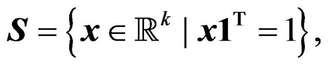 (1.9)
(1.9)
where  is the length
  vector with each entry equal to 1. Here
  is isomorphic to
  and
and  so we think of
 ![]() as a
as a  dimensional unit simplex, with the
  unit strategy vectors
 ![]() as its vertices. For each pair of strategy vectors
as its vertices. For each pair of strategy vectors  the payoff one receives from playing
 ![]() against
against ![]() is
is
 (1.10)
The best response set to any strategy vector  is the set of pure strategies
  such that
 (1.11)
The  th best response region
  is the set of all points in
  that have a best response set equal to
 , in other words
  is the set of points
  where
where
 (1.12)
Let us define a “division” of a subset of Euclidian space to be a collection of closed regions such that every point of the space lies within some region, and the interiors of any pair of distinct regions do not intersect. We say a division is convex when each of its regions is convex. Every  strategy game
  induces a division of
  into
into  convex best response regions
 , because every point of
  belongs to some best response region
 , and pairs of distinct best response regions only intersect at their boundaries.
Let  be the set of all points
  that can be written as
 (1.13)
for some  (where our sum takes into account that some elements may occur in
  several times). The set of points
  will be partitioned into different best response regions
  and the nature of this partition determines the update function
  of the regular automata that occurs when the game
  is used for a best response game on a
 ![]() regular graph. We say that the partition of
regular graph. We say that the partition of  into different best response regions
  is the best response partition of
  induced by the game
 .
.
Suppose we have a generic best response game , where
  is a regular degree
 ![]() graph. This will be a regular automata
graph. This will be a regular automata  where
where  is the strategy
  such that
 (1.14)
Consider for example the Hawk-Dove game discussed in the previous section. This is a two strategy game so our strategy space ![]() is the unit line. We can plot the payoffs one receives from playing strategy 1 or 2 against the different strategy vectors
is the unit line. We can plot the payoffs one receives from playing strategy 1 or 2 against the different strategy vectors  as shown in Figure 3. This induces a convex division of
 ![]() into two best response regions
into two best response regions  and
and . The update function
  is determined by considering how the points of
 (1.15)
are divided up into these best response regions. For example  so
so .
.
For a 3 strategy game the simplex ![]() is the unit triangle. Again we can plot the payoffs one receives from playing pure strategies against strategy vectors in
is the unit triangle. Again we can plot the payoffs one receives from playing pure strategies against strategy vectors in![]() . In Figure 4 (left) the x-y plane represents the different strategy vectors, and the z coordinate representing the payoffs one receives from employing different pure strategies against these vectors. Again this induces a division of the simplex
. In Figure 4 (left) the x-y plane represents the different strategy vectors, and the z coordinate representing the payoffs one receives from employing different pure strategies against these vectors. Again this induces a division of the simplex ![]() into convex best response regions.
into convex best response regions.
Theorem 1 
A partition of the points of  into
into  subsets
  is induced by the best response division associated with some
  strategy game
  if and
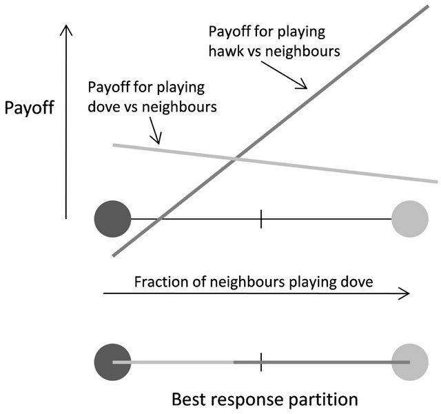
Figure 3. A plot showing the payoff received from using pure strategies against mixed strategies in the game described by Equation (1.5). The best response division is calculated by observing the pure strategy that scores best against each point of the strategy space.
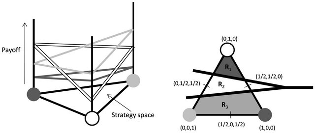
Figure 4. On the left is an illustration of how pure strategies score different payoffs against mixed strategies in three strategy games. On the right is the best response division associated with the game described by Equation (1.6).
only if the convex hulls of each pair of distinct subsets  and
and  do not intersect.
Theorem 1 allows us to determine when a given  state regular automata is a best response game. The proof is in the appendix and the remainder of this section describes the geometry of best response divisions in more detail. Given a non-singular payoff matrix
  we can find a division of the
  -dimensional space
  into (open) best response regions
 . First we will consider best response divisions of
 . Later we will consider how such divisions divide up the points of the simplex of attainable strategies
 (1.16)
For each pair  let
let  be the set of all
  where
where
 (1.17)
The hyperplane  is the set where the payoffs to pure strategies i and j are equal. Since M is nonsingular this hyperplane has dimension
 . The hyperplane divides
  into two regions, one where the payoff to pure strategy
  exceeds that to pure strategy
 , and the other where the payoff to pure strategy
exceeds that to pure strategy . Each of the
pairs  define such a dividing hyperplane. The set
![]() (1.18)
(1.18)
of all of these hyperplanes together divide up the space  into the
  distinct regions corresponding to the distinct orderings of the
  payoffs at each point. The best response region
  is the union of
  of these
  regions, and these are necessarily contiguous. The set of regions correspond to the orderings of
 , i.e. the permutations. The Cayley graph of the group
  under the generator set of transposition of adjacent elements corresponds to the adjacency of the
 . Each transposition corresponds to the crossing of a hyperplane where there is equality of the payoffs for the elements which are transposed.
Alternately we can consider the sets
 (1.19)
and  is the set of
  where the payoffs to the elements of
  are equal. Since
  is nonsingular there exists a unique value
 (1.20)
(A Nash equilibrium of the system.) Each  passes through
  and on one side the payoff to
  is greater than that to all the others, and on the other side it is less. We consider the set of
  rays consisting of
  and that part of
  where the payoff to
  is less than the payoff to the other strategies,
 . Since our matrix is non-singular the set of rays form a basis for the simplex. For some set
  the convex combination of the corresponding rays,
  is the set where there is equality of the payoffs to the set of payoffs indexed by the elements not in
 , all elements in
  having lower payoffs. The regions
  are the interiors of the (closed) regions generated by convex combinations of points from
 . Each of these
  closed regions is bounded by
  rays.
rays.
Thus we have that the division of the unit simplex into the  best response regions is simply achieved by taking a point in the hyperplane containing the unit simplex, and
  rays emanating from that point with the condition that the reflection of any ray in the central point lies in the convex hull of the other
  rays.
rays.
The converse of the above argument is simply that if we have a division of the hyperplane containing the unit simplex according to the above rule then we can find a unique matrix which corresponds to those rays. Of course in the context of a game on a circle there will be many sets of rays which produce the same best response regions, and thus many payoff matrices. Suppose then that we are given the specification of the rays as a set of linearly independent vectors  for
for  and form the matrix
  which has the columns equal to the
 , then we select any matrix
  with
with  column which have equal entries except for the diagonal entry which is smaller. Now we only require to find matrix
  such that
 (1.21)
i.e. , for this matrix M to provide us with an appropriate payoff matrix, though we may require to add a constant to all elements if we require payoffs to be positive.
Example. Suppose the rays from the central equilibrium value are such that the matrix  is given by
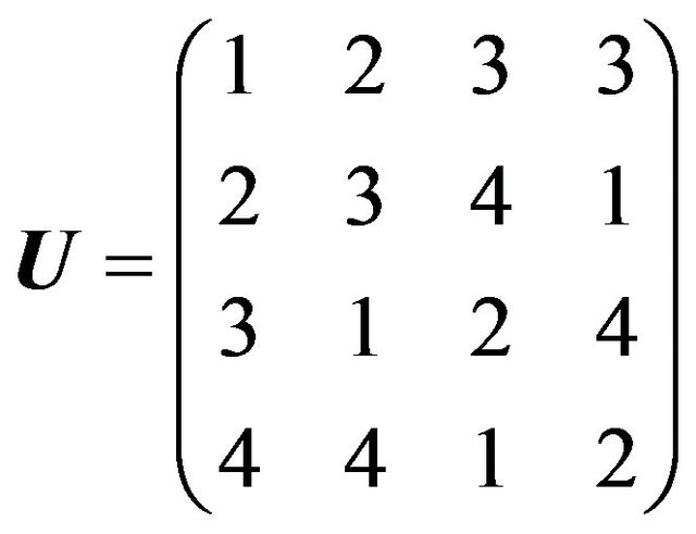
Note that the columns add to a constant but this is not required. Now we can select any appropriate matrix . For ease we take
 , where
  is the unit matrix. We have
and we can add 1 if we require positive entries.
3. Games on the Circle with 2 or 3 Strategies
We can apply Theorem 1 to enumerate the two strategy best response games on the circle. To do this we must simply list all the different possible ways to divide up our simplex![]() , the unit line, into two or less convex regions, with respect to the three points of
, the unit line, into two or less convex regions, with respect to the three points of —the lines two end points and the mid point.
There are only two ways of doing this, either all points belong to the same region or one end point belongs to one region and the other two points belong to the other. We can take each of these two unlabeled divisions and apply labels to the regions, deciding which best response regions they represent. We hence find that there are six non-identical two strategy best response game on the circle, three of which are permuationally distinct, meaning there are three fundamentally different types of two strategy best response games (see Table 1).
The first type are games where one strategy strictly dominates. These systems induce very dull dynamics with every vertex constantly playing the dominating strategy. Figure 1 depicts the dynamics of a game of the
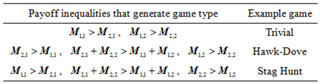
Table 1. The payoff inequalities describe the three types of two strategy game that induce fundamentally different dynamics in best response games on the circle.
second type. The dynamics induced correspond to Wolfram’s automata number 95. When the circle has even length there are two repelling fixed points, where no adjacent vertices share the same strategy. The system has many period two orbits which quickly attract other configurations. The third type of game corresponds to Wolfram’s automata number 160. When the circle has even length there is a repelling period two orbit—jumping between the two configurations with no adjacent vertices sharing the same strategy. The system has many fixed points which quickly attract other configurations.
We can use Theorem 1 again to enumerate the best response games on the circle with three strategies. Recall how the best response division depicted at the right of Figure 4 induces the dynamics depicted in Figure 2. Our theorem implies that any division of ![]() (which is the unit triangle) into three or less convex regions is induced by some game. The update function induced by such a division depends upon the way the six points of
(which is the unit triangle) into three or less convex regions is induced by some game. The update function induced by such a division depends upon the way the six points of  (the 3 vertices and 3 edge-midpoints of the triangle) are partitioned into these best response regions.
To enumerate all of the three strategy games we must simply list all the fundamentally different ways of dividing up ![]() into three or less convex regions with respect to the points of
into three or less convex regions with respect to the points of . There are 12 fundamentally different ways to perform such a division.
Each division ![]() induces an equivalence class, which is the set of best response divisions of
induces an equivalence class, which is the set of best response divisions of  which can be attained by taking
 ![]() and labeling the regions with different strategies-deciding which best response region each region of
and labeling the regions with different strategies-deciding which best response region each region of ![]() represents. By looking at the different labellings of the 12 divisions we find that there are 285 non-identical three strategy best response games on the circle, 52 of which are permutationaly distinct. We give space time plots of the 52 cases in the appendix (subsection 6.4), together with diagrams that show the divisions corresponding to the equivalence classes of the games.
represents. By looking at the different labellings of the 12 divisions we find that there are 285 non-identical three strategy best response games on the circle, 52 of which are permutationaly distinct. We give space time plots of the 52 cases in the appendix (subsection 6.4), together with diagrams that show the divisions corresponding to the equivalence classes of the games.
4. Games with More Strategies
Enumeration of best response games on the circle with more than three strategies is difficult to do in the same visual manner as above. The reason is that the simplex is high dimensional and the number of different convex divisions of the simplex with respect to  is large. Since the set of
  strategy best response games on the circle are a subset of the set of
  state regular automata one fruitful question to ask is when is a
  state regular automata on the circle not a
  strategy best response game?
We can think of each regular automata,
 , on a d regular graph
 , as inducing a partition of
  in a similar way to the way we did for best response games. To do this is that we think of our set of states as numbers
  and we think of each
  as a point
 (1.22)
in the simplex. We think of the points
 as being partitioned into
  subsets
  where
where  is the set of all points
  such that
 .
.
The converse of Theorem 1 is that a regular automata  is not a
 ![]() strategy best response game if and only if the partition of
strategy best response game if and only if the partition of  that
that
 induces has a distinct pair of sets
  and
and  with intersecting convex hulls.
So to answer our question, we should find all of the pairs of disjoint subsets  such the convex hulls of
  and
and  intersect. We call such an
  pair
pair  unacceptable because a
  state regular automata
  on a
on a ![]() regular graph is not a best response game if and only if
regular graph is not a best response game if and only if ![]() has a pair of states
has a pair of states , such that
 are
are  unacceptable.
Clearly if a pair  are such that there is a pair
  and
and  where
where  are
are  unacceptable, for
 , then
  are
are  unacceptable. Knowing this we can tighten the definition of unacceptable pairs, to lessen the number of objects we need to catalogue to determine whether or not a regular automata is a best response game.
We say that a pair  are fundamentally
  unacceptable if and only if
  are
are  unacceptable and
 ,
,  ,
,  we have that
  are
are  unacceptable implies
 and
and .
.
In other words a fundamentally unacceptable pair is an unacceptable pair that properly contains no other unacceptable pairs. So we arrive at Theorem 2.
Theorem 2 
A  state regular automata
  on a
on a ![]() regular graph is a best response game if and only if
regular graph is a best response game if and only if , for every pair of states
  of
of![]() , there does not exist a pair
, there does not exist a pair ,
, that is fundamentally
  unacceptable.
Our enumeration problem is hence transformed into the problem of finding the set of permuationally distinct fundamentally unacceptable pairs. The set of different convex partitions of  can be found by listing all the permuationally distinct partitions of
  and then filtering out those partitions which involve a pairs
  such that
 ,
,  is fundamentally
  unacceptable, for
 .
.
Let us consider the problem on the circle, when . There are no fundamentally
  unacceptable pair because
  cannot be split into two disjoint nonempty sets. The fundamentally
  unacceptable pairs can be found visually, the only permuationally distinct way one may choose two disjoint subsets
  and
and  of
of  such that the convex hulls of
  and
and  intersect is
and . The pair
 , where
 and
and  is hence the only permuationally distinct fundamentally
  unacceptable pair.
The set of fundamentally  unacceptable pairs can again be found visually. It is easy to see that, if the convex hulls of two disjoint sets of
 , in the unit triangle, intersect, then one of the two situations depicted in Figure 5 must have occurred.
For a pair of disjoint sets , let
, let  be the graph with a vertex set consisting of all
  such that
 ![]() is a member of a pair in
is a member of a pair in  or
or![]() , and edge set consisting of dark gray edges
, and edge set consisting of dark gray edges  and light gray edges
![]() . An alternating walk on such a graph
. An alternating walk on such a graph  is a walk on the edges of
  such that every edge traversed is a different colour to the previously traversed edge. An alternating cycle of such a graph is an alternating walk that finishes on the same vertex where it started returning along an edge of a different colour to the colour of the edge that the walk first traversed.
Lemma 1 A pair  is
is  unacceptable if and only if
  has an alternating cycle.
This leads to a result that allows us to completely cha-
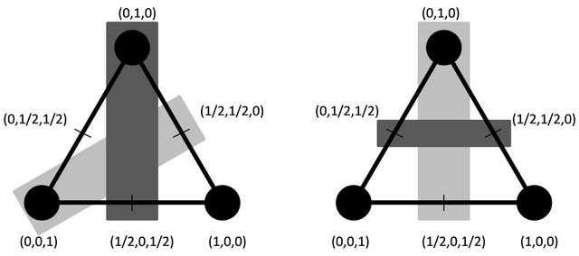
Figure 5. The two fundamentally  unacceptable pairs within the two dimensional simplex Δ. The left shows
 ,
,  , the right shows
  ,
, .
.
racterise the set of fundamentally  unacceptable graphs for generic
 . Recall that
  denotes the
 ![]() vertex circle graph, let
vertex circle graph, let  be a single vertex with a self loop. Let a
  vertex dumbbell graph
 , where
 , be the fusing of two circle graphs
 ![]() and
and  to the two end points of a line graph (by identifying/overlapping vertices) so that the resulting graph,
  , has
, has  vertices (see Figure 6). Note that when
 , the connecting line between the two circles in
  has no edges, and hence
  resembles a figure-eight in that it consists of two circles intersecting at one vertex.
Let a good colouring of a graph  be a colouring of its edges with dark gray and light gray such that, if a vertex
  only has two edges incident on it then the two edges are painted different colours and otherwise two edges incident on a vertex
 ![]() are painted different colours if and only if they do not lie on the same cycle of
are painted different colours if and only if they do not lie on the same cycle of .
.
Theorem 3  is fundamentally
  unacceptable if and only if one of the following conditions hold:
1)  and
and  is a good colouring of
 ;
;
2)  is even and
  is a good colouring of
  or
or  where
where  are even and such that
 ;
;
3)  is odd and
  is a good colouring of
  where
where  are even and such that
 .
.
Using Theorems 2 and 3 we can make an algorithm to check if a regular automata on the circle corresponds to a best response game and hence we can solve the problem of finding all of the fundamentally different 4 strategy best response games on the circle. The way we do this is to use a computer to generate the set of all four state degree 2 regular automata and then filter this set, removing those rules that do not correspond to best response games. We find that there are 143,524 non-identical four strategy games and 6041 permutationally distinct games.
5. Games on Other Graphs
When dealing with degree three graphs, the different update functions F that can occur correspond to convex divisions of ![]() with respect to the points of
with respect to the points of . With two strategies, we may enumerate the possible best re-

Figure 6. On the left is an illustration of . On the right is an illustration of
 . Both graphs have been given a good colouring.
sponse games by listing the different divisions of the unit line ![]() into
into  convex regions with respect to the points of
 . Using this approach one can determine the 5 permutationally distinct update functions F that could be induced by two strategy best response games on degree three graphs. Its important to note that the update rules found in this way could be evolved upon many different graph topologies. One could consider dynamics of the cube, the Peterson graph or any other degree three graph. The circle with self-linkage is the degree three graph obtained by taking a circle and linking each vertex to itself. Looking at best response games on the circle with self linkage is beneficial because the resulting one dimensional cellular automata can be visualised using space time plots. The permutationally distinct two strategy best response games running on the circle with self linkage correspond to rules Wolfram’s elementary cellular automata numbers 0, 23, 127, 128 and 232. One may enumerate the different three strategy games on degree three graphs in a similar manner by listing the different ways to cut up the unit triangle into convex regions with respect to the points of
 . Using this method one finds that there are 82 fundamentally different three strategy best response games on degree three graphs.
These methods can be applied to enumerate the number of  strategy games on degree
 ![]() graphs. Such an enumeration seems difficult to do for generic
graphs. Such an enumeration seems difficult to do for generic  and
and![]() . Theorem 1 provides a way to do such an enumeration in theory but with no result like Theorem 3 (which allows us to quickly filter out unviable regular automata) the computation would be slow for
. Theorem 1 provides a way to do such an enumeration in theory but with no result like Theorem 3 (which allows us to quickly filter out unviable regular automata) the computation would be slow for .
.
Our results can be extended to deal with non-regular graphs. Suppose we have a graph  and
and  is the set of all
  such that there is a vertex of
  with degree
 . To enumerate the different best response games on
  one must simply list all the different ways to divide
 ![]() into
into  or less convex regions with respect to the points of
![]() .
.
REFERENCES
- J. von Neumann and O. Morgenstern, “Theory of Games and Economic Behavior,” Princeton University Press, Princeton, 1944.
- J. Nash, “Non-Cooperative Games,” The Annals of Mathematics, Vol. 54, No. 2, 1951, pp. 286-295. doi:10.2307/1969529
- J. Maynard Smith, “Evolution and the Theory of Games,” Cambridge University Press, Cambridge, 1982. doi:10.1017/CBO9780511806292
- G. Szabo and J. Fath, “Evolutionary Games on Graphs,” Physics Reports, Vol. 446, No. 4, 2007, pp. 97-216. doi:10.1016/j.physrep.2007.04.004
- F. Santos, J. Pacheco and T. Lenaerts, “Evolutionary Dynamics of Social Dilemas in Structured Heterogeneous Populations,” Proceedings of the National Academy of Sciences of the United States of America, Vol. 103, No. 9, 2006, pp. 3490-3494. doi:10.1073/pnas.0508201103
- M. Nowak and R. May, “Evolutionary Games and Spatial Chaos,” Nature, Vol. 359, No. 6398, 1992, pp. 826-829. doi:10.1038/359826a0
- R. Southwell, J. Huang and B. Shou, “Modelling Frequency Allocation with Generalized Spatial Congestion Games,” IEEE ICCS, 2012.
- R. Southwell and J. Huang, “Convergence Dynamics of Resource-Homogeneous Congestion Games,” GameNets, 2011.
- R. Southwell, Y. Chen, J. Huang and Q. Zhang, “Convergence Dynamics of Graphical Congestion Games,” Springer, Berlin, Heidelberg, 2012, pp. 31-46.
- R. Southwell, X. Chen and J. Huang, “Quality of Service Satisfaction Games for Spectrum Sharing,” IEEE INFOCOM—Mini Conference, 2013.
- R. Southwell and C. Cannings, “Games on Graphs That Grow Deterministically,” GameNets, 2009, pp. 347-356.
- R. Southwell and C. Cannings, “Some Models of Reproducing Graphs: I Pure Reproduction,” Applied Mathematics, Vol. 1, No. 3, 2010, pp. 137-145.
- R. Southwell and J. Huang, “Complex Networks from Simple Rewrite Systems,” arXiv Preprint arXiv:1205. 0596, 2012.
- R. Southwell and C. Cannings, “Exploring the Space of Substitution Systems,” Complex Systems, 2013.
- R. Southwell and C. Cannings, “Some Models of Reproducing Graphs: III Game Based Reproduction,” Applied Mathematics, Vol. 1, No. 5, 2010, pp. 335-343.
- R. Southwell and C. Cannings, “Some Models of Reproducing Graphs: Ii Age Capped Vertices,” Applied Mathematics, Vol. 1, No. 4, 2010, pp. 251-259.
- S. Berninghaus and U. Schwable, “Conventions, Local Interaction, and Automata Networks,” Evolutionary Economics, Vol. 6, No. 3, 1996, pp. 297-312.
- S. Berninghaus and U. Schwable, “Evolution, Interaction, and Nash Equilibria,” Journal of Economic Behavior and Organization, Vol. 29, No. 1, 1996, pp. 57-85. doi:10.1016/0167-2681(95)00051-8
- C. Cannings, “The Majority Game on Regular and Random Networks,” GameNets, 2009, pp. 1-16.
- S. Wolfram, “A New Kind of Science,” Wolfram Media, 2002.
- P. Kurka, “Topological and Symbolic Dynamics,” Societe Mathematique de France, 2003.
6. Appendix
6.1. Proof of Theorem 1
Any game  will induce a division of the extended strategy space
  into best response regions
 . To show these best response region are convex, consider two points
 ![]() and
and ![]() within
within , then
 and
and ,
,
 , by definition. Since
  is a linear mapping any convex combination
 , for
, for  will be such that
 ,
,
 . This means
  also lies within the best response region
 . So every best response region
  is convex. This means our game induces partition of
  into best response regions
  , such that the convex hulls of any two sets
  do not overlap.
Proving the converse is more involved.
Suppose we have a partition of the points of  into
into  sets
sets  such that the convex hulls of each pair of sets do not overlap. There will be a family of appropriate divisions of
 , into
  convex open sets
 , that generate such a partition of
  in that
 ,
, .
.
Each such division, where every region  has non zero volume, must be generated by a set of dividing hyperplanes, which is a set of
  dimensional hyperplanes that cut up the space into different regions. Each
  is a polyhedral set and every
  dimensional face of
  is the intersection of the closure of
  with one of its neighboring regions. The set of dividing hyperplanes which generates such a division is the set of affine hulls of all such faces of all regions.
Among our family of appropriate divisions there will be a division of  into
into  non-zero volume, convex sets
  with the property that each set of
  dividing hyperplanes involved in this division will meet at a single point, we will call such a division proper. It is a well known result that almost every arrangement of
  hyperplanes of dimension
  in
in  will have a common point, such a point will always exist provided no two of these hyperplanes have parallel subspaces. Any division can be made proper by doing an infinitesimal perturbation of the positioning of the dividing hyperplanes involved. Since the points of
  are distantly spaced such a perturbation will not effect the way
  is partitioned up. This means an appropriate proper division exists.
Suppose  is a region within an appropriate proper division. We shall use a proof by contradiction to show that
  has a finite extreme point (a vertex). Suppose (falsely) that
  does not have a finite extreme point.
Let  denote the closure of
 . Any closed convex set, like
 , with no finite extreme point, must contain a line
 ![]() (extending infinitely in both directions). Any translation of
(extending infinitely in both directions). Any translation of ![]() that intersects with
that intersects with  must also be contained within
 . Let
. Let  be a region adjacent to
 . Any translation of
 ![]() that intersects with
that intersects with  must be contained within
 . This means any translation of
 ![]() that intersects
that intersects  must be contained within
 . This argument can be continued to show that every region contains a translation of
 ![]() and every dividing hyperplane contains a translation of
and every dividing hyperplane contains a translation of![]() . This contradicts our assumption that the division is proper because such an arrangement of dividing hyperplanes cannot meet at a point. Every
. This contradicts our assumption that the division is proper because such an arrangement of dividing hyperplanes cannot meet at a point. Every  dimensional cross section of our hyperplane arrangement attained by slicing perpendicular to
 ![]() will look the same (irrespective of how far along
will look the same (irrespective of how far along ![]() one chooses to slice) so there cannot be a point where all the dividing hyperplanes meet. This contradiction implies every region
one chooses to slice) so there cannot be a point where all the dividing hyperplanes meet. This contradiction implies every region  must have a vertex.
Since  is
is  dimensional a vertex of
  must be the intersection of at least
  of its faces. Each of
  ‘s faces is
  for some neighbouring region
 . There are only
  regions so
  can have at most
  faces. Hence
  has just one vertex
![]() , and
, and ![]() is the intersection of the closures of all
is the intersection of the closures of all  regions. Let
  be the intersection of the closures of every region except
 , it follows that
  will be a one dimensional ray that is a common one dimensional edge of every region except
 . There will be
  such one dimensional rays
 , that all meet at
 ![]() and every region
and every region  will be the interior of the convex hull of
 . Each ray must lie outside of the convex hull of the other
  rays (otherwise the interior of two regions would intersect and we would not have a division). An equivalent way to say this is that the reflection of any ray in
 ![]() lies within the convex hull of the other
lies within the convex hull of the other  rays.
rays.
Since our regions meet at a central point with  emanating rays (that meet the appropriate conditions) we can use the results from section 0.2 to construct a nonsingular payoff matrix
  which generates our convex division. Under the game with payoff matrix
  the
the  th best response region
  will be equal to the convex region
 ,
, . □
. □
6.2. Proof of Lemma 1
We will show that a pairs unacceptability implies the presence of an alternating cycle. Suppose that
 is a
is a  unacceptable pair, then by definition, there must exist subsets
 ,
, 
and sets of positive reals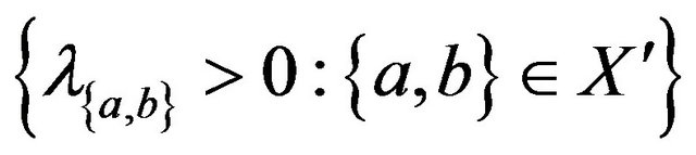 ,
,
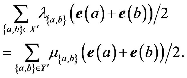
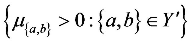 such that
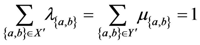 (1.23)
and
 (1.24)
Now consider the graph  with each dark gray edge
  weighted with the constant
  and each light gray edge
  weighted with the constant
 . The sum of the weights of the dark gray edges incident upon any vertex will be equal to the sum of the weights of the light gray edges that are incident upon that vertex (where self edges are counted as being incident twice). Suppose
 ![]() is the minimal weight on any edge of
is the minimal weight on any edge of , let us multiply all of the weights of
 ’s edges by
 , so that all of the weights will be at least 3.
Now start on any vertex of , and walk along a dark gray edge, when the walk traverses an edge, reduce the weight of that edge by 1. After traversing a dark gray edge, let the walk traverse a light gray edge, then a dark gray edge, then a light gray... and continue in this manner, reducing the weight of every traversed edge. When an edge reaches weight
  it disappears and can no longer be used.
Every vertex must have at least two incident edges, one of each colour and such a walk is allowed to traverse each edge at least twice. Moreover, every time the walk approaches a vertex with an edge of one colour, it will be able to leave the vertex with an edge of the other colour (at least this will be true until an edge has been traversed twice). Clearly such a walk will be allowed to continue, in an alternating manner, until an edge is traversed three times. After an edge has been traversed three times it follows that some vertex ![]() must have been visited three times. This implies that an alternating cycle has been generated. To see this suppose, without loss of generality, that our walk first leaves
must have been visited three times. This implies that an alternating cycle has been generated. To see this suppose, without loss of generality, that our walk first leaves ![]() along a dark gray edge. If the walk returns to
along a dark gray edge. If the walk returns to![]() , for the first time, along a light gray edge then an alternating cycle has clearly been generated. If, on the other hand, the walk returns to
, for the first time, along a light gray edge then an alternating cycle has clearly been generated. If, on the other hand, the walk returns to![]() , for the first time along a dark gray edge then it must leave
, for the first time along a dark gray edge then it must leave![]() , for the second time, along a light gray edge. When the walk returns to
, for the second time, along a light gray edge. When the walk returns to ![]() for the second time it will complete an alternating cycle. To see this note that whatever the colour of the edge which the walk uses to return to
for the second time it will complete an alternating cycle. To see this note that whatever the colour of the edge which the walk uses to return to ![]() for the second time, the walk will have used an edge of the opposite colour to leave
for the second time, the walk will have used an edge of the opposite colour to leave ![]() previously. This shows a pairs unacceptability implies the presence of an alternating cycle.
previously. This shows a pairs unacceptability implies the presence of an alternating cycle.
To see the converse suppose that the graph  contains an alternating cycle
  with
with ,
, . Now
. Now  let
let  be the number of times that the edge
  is traversed in the alternating cycle
 . Similarly
  let
let  be the number of times that the edge
  is traversed in the alternating cycle
 . We refer to
  as the weight of the dark gray edge
  and we refer to
  as the weight of the light gray edge
 .
.
Our alternating cycle will be such that the number of traversals of dark gray edges must be equal to the number of traversals of light gray edges, and hence our coefficients will be such that
 (1.25)
for some constant .
.
The alternating cycle will be a walk such that every time a vertex is approached along an edge of one colour the walk will leave the vertex along an edge of another colour and each edge  of
of  is traversed by this walk a number of times equal to its weight. It follows that, for every vertex
 ![]() of
of , the sum of the weights of
![]() ’s incident dark gray edges is equal to the sum of the weights of
’s incident dark gray edges is equal to the sum of the weights of![]() ’s incident light gray edges (where self edges are counted as being incident twice).
’s incident light gray edges (where self edges are counted as being incident twice).
Hence we get
 (1.26)
so we can divide all of our parameters  and
and  by our constant
  to get the set of convex coefficients which describe a point where the convex hull of
 and
and  intersect. □
6.3. Proof of Theorem 3
Suppose  is fundamentally
  unacceptable, then according to the definition of fundamentally unacceptable pairs and lemma 1,
  is an alternating cycle, and hence must be connected. Moreover there can only be one recolouring of the edges of
 , then is an alternating cycle (that recolouring which just swaps the colours of every edge). If this were not so then
  would contain more than one fundamentally different alternating cycle, and hence would not be fundamentally unacceptable.
Now suppose that  has an even cycle C on more than three vertices. C can be recoloured to be an alternating cycle, and this means that
  consists of exactly C and nothing more. Note that C is a good colouring a circle graph on an even number of vertices.
Next suppose that  has no even cycles, and at most one odd cycle. In this case
  can not be fundamentally
  unacceptable. To see this consider a walk which is an alternating cycle. Such a walk must traverse a cycle of the graph. The walk cannot take place on a purely linear graph (i.e. a line graph) because this would imply that the walk must change direction at some point -back tracking along the edge just used, but this violates our requirement that the colours of edges used alternate. Now let us (falsely) suppose that our
  does have a walk which is an alternating cycle. Since our walk is required to traverse a cycle of
  we can assume (without loss of generality) that the walk begins at a vertex
 ![]() on the odd cycle of
on the odd cycle of  and immediately traverses the cycle. When the walk returns to
![]() , for the first time, it will do so along an edge of the same colour as the first edge traversed in the walk. To complete an alternating cycle the walk must return to
, for the first time, it will do so along an edge of the same colour as the first edge traversed in the walk. To complete an alternating cycle the walk must return to ![]() along a different colour. Clearly traversing the odd cycle again is not going to achieve this. The only other way to try (in our efforts to form an alternating cycle) is to have the walk leave the odd cycle, to visit other vertices of
along a different colour. Clearly traversing the odd cycle again is not going to achieve this. The only other way to try (in our efforts to form an alternating cycle) is to have the walk leave the odd cycle, to visit other vertices of . This cannot be done however because
  only holds one cycle. Once our walk leaves this cycle it will have no way to return except to backtrack, which we have already shown is not allowed.
Now the only other possible case is that  contains no even cycles and at least two odd cycles
  and C. Since
  is connected there must be a linear path
  (a sequence of end to end edges forming a line graph) between
  and C. Now
  can be given an edge recolouring (the good colouring of
 ) that is an alternating cycle. We shall construct such a cycle by describing a walk (it will be clear that
 ’s edges can be coloured in such a way that the edge colours alternate on this walk). Suppose our walk starts off at the intersection of
  and
and  (the vertex
  of
of  which is an point of the line graph
 ). Suppose the walk begins by traversing
 , starting off with a dark gray edge. After traversing
 , the walk will return to
  along a dark gray edge. Next the walk travels along a light gray edge of P towards
 . Suppose the walk continues traveling along P until it reaches the other end point, e, of P (which intersects with C). The walk then moves around C, returning to
 ![]() on the same colour edge by which it set off (on C), and then the walk travels back along P, to
on the same colour edge by which it set off (on C), and then the walk travels back along P, to . When the walk returns to
  it will do so along a light gray edge, thus completing the alternating cycle. So we have shown that if
  contains more than one odd cycle, then
  must exactly be of the form
 , which is exactly the form of a dumbbell graph
  where
where  are even and such that
 . Such a graph will only have one fundamentally different alternating cycle, which can be found by doing a good colouring of it.
So we have shown that all the graphs associated with fundamentally  unacceptable pairs
  lie in the set
  of graphs described in the theorem (even length circle graphs and dumbbell graphs with odd cycles). All that remains is to show that there are not any graphs within this set that are not
  unacceptable. We know that each of these graphs has at most one fundamentally different alternating cycle and no unnecessary extra structure, so all that is left is to show that no graph in
  has a proper subgraph that is a member of
  for
for . For a dumbbell graph with two odd cycles, this is obvious since every proper subgraph of it is neither a dumbbell graph, nor a circle graph of even length. Similarly no proper subgraph of a circle graph is a circle graph or a dumbbell graph. □
6.4. The Different Three Strategy Games on the Circle
In this subsection we give example space time plots (from random initial conditions) showing the dynamics of each of the 52 non-identical best response games on the circle (see Section 3). We group these plots together with the diagrams that show the unlabeled partitions of  which can be coloured to yield their best response partitions (see Figures 7-14).
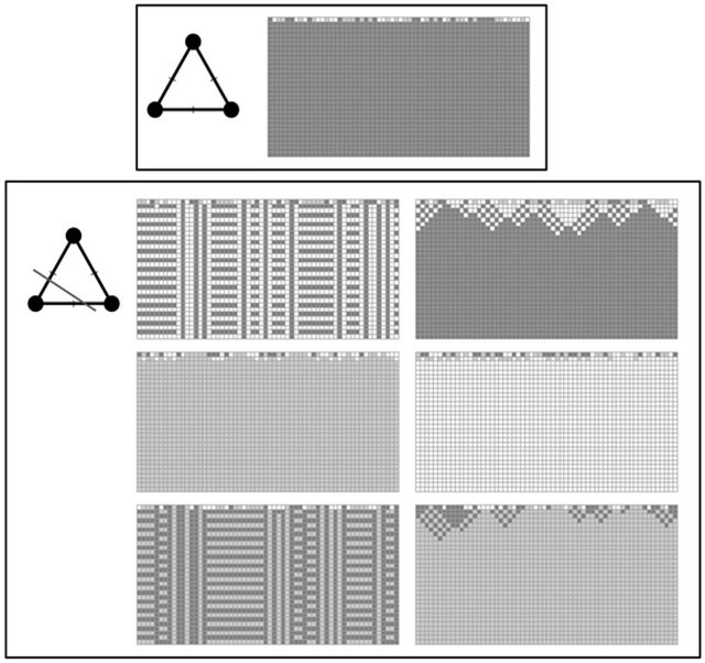
Figure 7. Diagrams of partitions 1 and 2 of T2, and spacetime plots of the associated best response games.
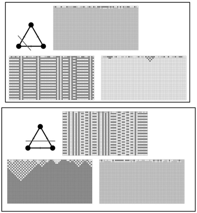
Figure 8. Diagrams of partitions 3 and 4 of T2, and spacetime plots of the associated best response games.

Figure 9. Diagrams of partitions 5 and 6 of T2, and spacetime plots of the associated best response games.
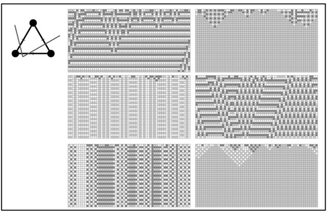
Figure 10. A Diagram of partition 7 of T2, and space-time plots of the associated best response games.
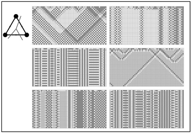
Figure 11. A Diagram of partition 8 of T2, and space-time plots of the associated best response games.

Figure 12. A Diagram of partition 9 of T2, and space-time plots of the associated best response games.
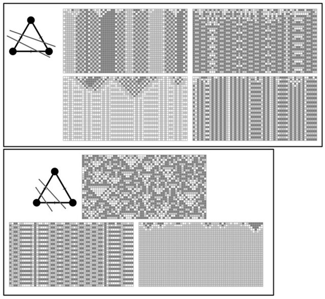
Figure 13. Diagrams of partitions 10 and 11 of T2, and space-time plots of the associated best response games.
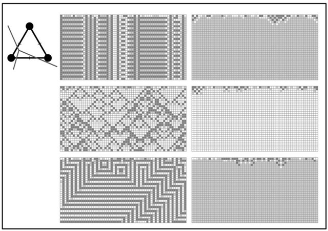
Figure 14. A Diagram of partition 12 of T2, and space-time plots of the associated best response games.