ABSTRACT

The Kuhn-Tucker theorem in nondifferential form is a well-known classical optimality criterion for a convex programming problems which is true for a convex problem in the case when a Kuhn-Tucker vector exists. It is natural to extract two features connected with the classical theorem. The first of them consists in its possible “impracticability” (the Kuhn-Tucker vector does not exist). The second feature is connected with possible “instability” of the classical theorem with respect to the errors in the initial data. The article deals with the so-called regularized Kuhn-Tucker theorem in nondifferential sequential form which contains its classical analogue. A proof of the regularized theorem is based on the dual regularization method. This theorem is an assertion without regularity assumptions in terms of minimizing sequences about possibility of approximation of the solution of the convex programming problem by minimizers of its regular Lagrangian, that are constructively generated by means of the dual regularization method. The major distinctive property of the regularized Kuhn-Tucker theorem consists that it is free from two lacks of its classical analogue specified above. The last circumstance opens possibilities of its application for solving various ill-posed problems of optimization, optimal control, inverse problems.

1. Introduction

We consider the convex programming problem

(P)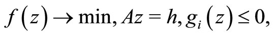

where is a convex continuous functional, is a linear continuous operator, is a fixed element, , , are convex functionals, D is a convex closed set, and Z and H are Hilbert spaces. It is well-known that the Kuhn-Tucker theorem in nondifferential form (e.g. see [1-3]) is the classical optimality criterion for Problem (P). This theorem is true if Problem (P) has a Kuhn-Tucker vector. It is stated in terms of the solution to the convex programming problem, the corresponding Lagrange multiplier, and the regular Lagrangian of the optimization problem (here, “regular” means that the Lagrange multiplier for the objective functional is unity).

Note two fundamental features of the classical Kuhn-Tucker theorem in nondifferential form (e.g. see [4-7]). The first feature is that this theorem is far from being always “correct”. If the regularity of the problem is not assumed, then, in general, the classical theorem does not hold even for the simplest finite-dimensional convex programming problems. In particular, the corresponding one-dimensional example can be found in [7] (see Example 1 in [7]). For convex programming problems with infinitedimensional constraints, the nonvalidity of this classical theorem can be regarded as their characteristic property. In this case a simple meaningful example can be found in [7] (see Example 2 in [7]) also.

The second important feature of the classical KuhnTucker theorem is its instability with respect to perturbations of the initial data. This instability occurs even for the simplest finite-dimensional convex programming problems. The following problem can be a particular example.

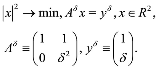
Example 1.1. Consider the minimization of a strongly convex quadratic function of two variables on a set specified by an affine equality constraint:

(1)

The exact normal solution is. The dual problem for (1) has the form

where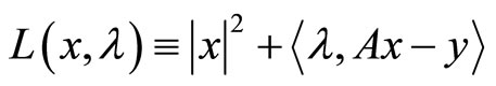         

and      .

Its solutions are the vectors. It is easy to verify that every vector of this form is a Kuhn-Tucker vector of problem (1). For consider the following perturbation of problem (1)

(2)

The corresponding dual problem

has the solution.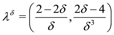

According to the classical Kuhn-Tucker theorem, the vector

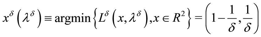
is a solution to perturbed problem (2). At the same time, this vector is an “approximate” solution to original system (1), and no convergence to the unique exact solution occurs as.

It is natural to consider the above-mentioned features of the classical Kuhn-Tucker theorem in nondifferential form as a consequence of the classical approach long adopted in optimization theory. According to this approach, optimality conditions are traditionally written in terms of optimal elements. At the same time, it is well-known that optimization problems and their duals are typically unsolvable. The mentioned above examples from [7] show that the unsolvability of dual problems fully reveals itself even in very simple (at first glance) convex programming problems. On the one hand, optimality conditions for such problems cannot be written in terms of optimal elements. On the other hand, even if they can, the optimal elements in these problems are unstable with respect to the errors in the initial data, which is demonstrated by Example 1.1. This fact is a fundamental obstacle preventing the application of the classical optimality conditions to solving practical problems. An effective way of overcoming the two indicated features of the classical Kuhn-Tucker theorem (which can also be regarded as shortcomings of the classical approach based on the conventional concept of optimality) is to replace the language of optimal elements with that of minimizing sequences that is sequential language. In many cases this replacement fundamentally changes the situation: the theorems become more general, absorb the former formulations, and provide an effective tool for solving practical problems.

So-called regularized Kuhn-Tucker theorem in nondifferential sequential form was proved for Problem (P) with strongly convex objective functional and with parameters in constraints in [7]. This theorem is an assertion in terms of minimizing sequences (more precisely, in terms of minimizing approximate solutions in the sense of J. Warga) about possibility of approximation of the solution of the problem by minimizers of its regular Lagrangian without any regularity assumptions. It contains its classical analogue and its proof is based on the dual regularization method (see, e.g. [4-7]). The specified above minimizers are constructively generated by means of this dual regularization method. A crucially important advantage of these approximations compared to classical optimal Kuhn-Tucker points (see Example 1.1.) is that the former are stable with respect to the errors in the initial data. This stability makes it possible to effectively use the regularized Kuhn-Tucker theorem for practically solving a broad class of ill-posed problems in optimization and optimal control, operator equations of the first kind, and various inverse problems.

In contrast to [7], in this article we prove the regularized Kuhn-Tucker theorem in nondifferential sequential form for nonparametric Problem (P) in case the objective functional is only convex and the set D is bounded. Just as in [7], its proof is based on the dual regularization method. Simultaneously, the dual regularization method is modified here to prove the regularized Kuhn-Tucker theorem in the case of convex objective functional.

This article consists of an introduction and four main sections. In Section 2 the convex programming problem in a Hilbert space is formulated. Section 3 contains the formulation of the convergence theorem of dual regularization method for the case of a strongly convex objective functional including its iterated form and the proof of the analogous theorem when the objective functional is only convex. In turn, in Section 4 we give the formulation of the stable sequential Kuhn-Tucker theorem for the case of a strongly convex objective functional. Besides, here we prove the theorem for the same case but in iterated form and in the case of the convex objective functional also. Finally, in Section 5 we discuss possible applications of the stable sequential Kuhn-Tucker theorem in optimal control and in ill-posed inverse problems.

2. Problem Statement

Consider the convex programming Problem (P) and suppose that it is solvable. Its solutions we denote by. We also assume that

where is a constant and

.

Below we use the notations:

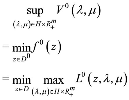
Define the concave dual functional called the value functional

and the dual problem

(3)

In what follows the concept of a minimizing approximate solution to Problem (P) plays an important role. Recall that a sequence, , is called a minimizing approximate solution to Problem (P) if, for, and. Here is the generalized infimum:

If f is a strongly convex functional and also if D is a bounded set, can be written as

Recall that in this case the Kuhn-Tucker vector of Problem (P) is a pair such that

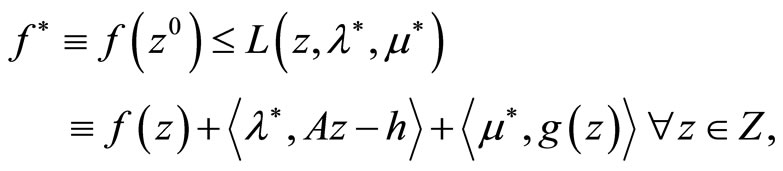
where is a solution to (P). It is well-known that every such Kuhn-Tucker vector is the same as a solution to the dual problem (3), and combined with constitutes a saddle point of the Lagrangian

.

3. Dual Regularization Algorithm

In this section we consider dual regularization algorithm for solving Problem (P) which is a stable with respect to perturbations of its input data.

3.1. The Original and Perturbed Problems

Let F be the set formed of all collections of initial data for Problem (P). Each collection consists of a functional f, which is continuous and convex on D, of a linear continuous operator A, an element h and functionals, that are continuous and convex on D. Moreover, it holds that

where the constant L_M is independent of the collection. If the objective functional of Problem (P) is strongly convex, then a functional f in each collection is continuous and strongly convex on D and has the constant of strong convexity that is independent of the collection.

Furthermore, we define collections and of unperturbed and perturbed data, respectively:

and       where characterizes the error in initial data and is a fixed scalar. Assume that

(4)

where is independent of and

.

Denote by (P⁰) Problem (P) with the collection of unperturbed initial data. Assume that (P⁰) is a solvable problem. Since

is a convex and closed set, we denote the unique solution of Problem (P⁰) in the case of strongly convex by. The same notation we leave for solutions of Problem (P⁰) in the case of convex also.

The construction of the dual algorithm for Problem (P⁰) relies heavily on the concept of a minimizing approximate solution in the sense of J. Warga [8]. Recall that a minimizing approximate solution for this problem is a sequence, such that

where and nonnegative scalar sequences, , converge to zero. Here is the generalized infimum for Problem (P⁰) defined in Section 2, and

.

It is obvious that, in general, where is the classical value of the problem. However, for Problem (P⁰) defined above, we have. Also, we can assert that every minimizing approximate solution of Problem (P⁰) obeys the limit relation

both in the case of convex and in the case of strongly convex.

Since the initial data are given approximately, instead of (P⁰) we have the family of problems

          

depending on the “error”.

Define the Lagrange functional

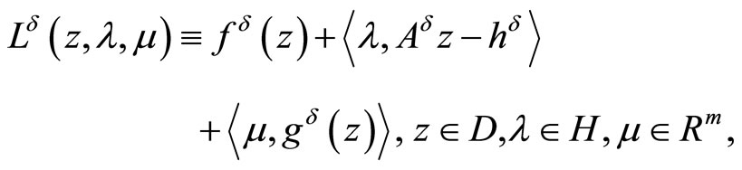
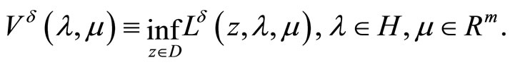
and the concave dual functional (value functional)

If the functional f is strongly convex, then due to strong convexity of the continuous Lagrange functional, for all, where

the value is attained at a unique element.

If D is a bounded set, then obviously the dual functional is defined and finite for all elements. When the functional f is convex, in the last case the value is attained at elements of the non-empty set

.

Denote by the unique point that furnishes the maximum to the functional

on the set.

Assume that the consistency condition

(5)

is fulfilled.

3.2. Dual Regularization in the Case of a Strongly Convex Objective Functional

In this subsection we formulate the convergence theorem of dual regularization method for the case of strongly convex objective functional of Problem (P⁰). The proof of this theorem can be found in [7].

Theorem 3.1. Let the objective functional of Problem (P) is strongly convex and the consistency condition (5) be fulfilled. Then, regardless of whether or not the Kuhn-Tucker vector of Problem (P⁰) exists, it holds that

Along with the above relations, it holds that

and, as a consequence,

(6)

If the dual problem is solvable, then it also holds that

where is the solution to the dual problem with minimal norm.

If the strongly convex functional is subdifferentiable in the sense of convex analysis on the set D, then it also holds that

In other words, regardless of whether or not the dual problem is solvable, the regularized dual algorithm is regularizing one in the sense of [9].

3.3. Iterative Dual Regularization in the Case of a Strongly Convex Objective Functional

In this subsection we formulate the convergence theorem of iterative dual regularization method for the case of strongly convex objective functional of Problem (P⁰). It is convenient for practical solving similar problems. The proof of this theorem can be found in [4].

We suppose here, that the set D is bounded and use the notation

where

is the sequence generated by dual regularization algorithm of Theorem 3.1. in the case,. Here is an arbitrary sequence of positive numbers converging to zero. Suppose that the sequence is constructed according to the iterated rule

(7)

where,

and the sequences, , obey the consistency conditions

(8)

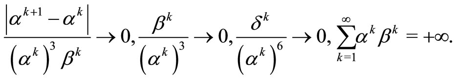
The existence of sequences and, , satisfying relations (8) is easy to verify. For example, we can use and.

Then, as it is shown in [4], the limit relations

(9)

hold and, as consequence, we have

(10)

Besides, if the strongly convex functional is subdifferentiable at the points of the set D, then we have also

The specified circumstances allow us to transform Theorem 3.1. into the following statement.

Theorem 3.2. Let the objective functional of Problem (P⁰) is strongly convex, the set D is bounded and the consistency conditions (8) be fulfilled. Then, regardless of whether or not the Kuhn-Tucker vector of Problem (P⁰) exists, it holds that

Along with the above relations, it holds that

and, as a consequence,

If the dual problem is solvable, then it also holds that

where is the solution to the dual problem with minimal norm.

If the strongly convex functional is subdifferentiable (in the sense of convex analysis) on the set D, then it also holds that

3.4. Dual Regularization in the Case of a Convex Objective Functional

In this subsection we prove the convergence theorem of dual regularization method for the case of bounded D and convex objective functional of Problem (P⁰).

Below, an important role is played by the following lemma, which provides an expression for the superdifferential of concave value function, in the case of a convex objective functional and a bounded set D. Here, the superdifferential of a concave function (in the sense of convex analysis) is understood as the subdifferential of the convex functional taken with an opposite sign. The proof is omitted, since it can be found for a more general case in [4].

Lemma 3.1. The superdifferential (in the sense of convex analysis of the concave functional at a point is expressed by the formula

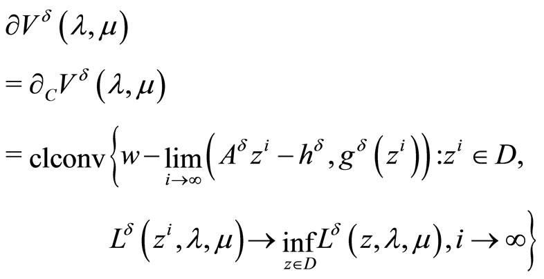
where is the generalized Clarke gradient of at, and the limit is understood in the sense of weak convergence in.

Further, first of all we can write the inequality

for an element

.

Then, taking into account Lemma 3.1. we obtain

(11)

where is such sequence that

Suppose without loss of generality that the sequence converges weakly, as, to an element belonging obviously to the set

Due to weak lower semicontinuity of the convex continuous functionals and boundedness of D we obtain from (11) the following inequality

where is some subsequence of the sequence.

To justify this inequality we have to note that in the case for some k the limit relation

holds despite the fact that the sequence converges only weakly to. This circumstance is explained by specific of Lagrangian (it is the weighed sum of functionals) and the fact that the sequence is a minimizing one for it.

As consequence of the last inequality, we obtain

(12)

(13)

(14)

In turn, the limit relations (12)-(14) and boundedness of D lead to the equality

(15)

Further, we can write for any

the following inequalities

From here, due to the estimates (4), we obtain

or

or

or

or, because of the equality (15)

or

From the last estimate it follows that

where

.

Thus, we derive the following limit relations

(16)

The limit relations (12)-(14), (16) give the possibility to write

(17)

Further, let us denote by

any weak limit point of the sequence

,.

Then, because of the limit relations (17) and the obvious inequality

we obtain

and, as consequence, due to boundedness of D

Simultaneously, since

and the inequality

holds, we can write for any due to the limit relation (15)

From the last limit relation, the consistency condition (5), the estimate (4) and boundedness of D we obtain

or

Thus, due to boundedness of D and weak lower semicontinuity of we constructed the family of depending on elements such that

and simultaneously

where any weak limit point of any sequence , is obviously a solution of Problem (P⁰).

Along with the construction of a minimizing sequence for the original Problem (P⁰), the dual algorithm under discussion produces a maximizing sequence for the corresponding dual problem. We show that the family

is the maximizing one for the dual problem, i.e. the limit relation

(18)

holds.

First of all, note that due to boundedness of D the evident estimate

(19)

is true with a constant which depends on

but not depends on.

Since

we can write, thanks to (19), the estimates

whence we obtain

From here, we deduce, due to the consistency condition (5) and limit relations (16), that for any fixed and for any fixed there exists such for which the estimate

(20)

holds.

Let us, suppose now that the limit relation (18) is not true. Then there exists such convergent to zero a sequence that the inequality

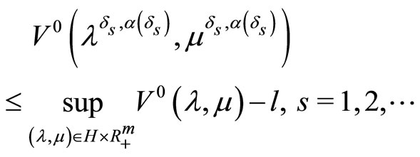
is fulfilled for some.

Since

for, we deduce from the last estimate that for all sufficiently large positive M the inequality

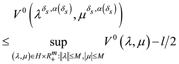
takes a place. This estimate contradicts to obtained above estimate (20). The last contradiction proves correctness of the limit relation (18).

At last, we can assert that the duality relation

(21)

for Problem (P⁰) holds. Indeed, similar duality relation is valid due to Theorem 3.1. (see relation (6)) for the problem

, with strongly convex objective functional. Writing this duality relation and passing to the limit as we get because of boundedness of D the duality relation (21).

In turn, from the duality relation (21), the estimate (19) and the limit relation (18) we deduce the limit relation

So, as a result of this subsection, the following theorem holds. To formulate it, introduce beforehand the notations

Theorem 3.3. Let the objective functional of Problem (P⁰) is convex and the consistency condition (5) be fulfilled. Then, regardless of whether or not the Kuhn-Tucker vector of Problem (P⁰) exists, it holds for some

that

(22)

Along with the above relations, it holds that

(23)

If the dual problem is solvable, then it also holds that

where          

is the solution to the dual problem with minimal norm.

4. The Stable Sequential Kuhn-Tucker Theorem

At first, in this section we give the formulation of the stable sequential Kuhn-Tucker theorem for the case of strongly convex objective functional. Next we prove the corresponding theorem in a form of iterated process in the same case and, at last, prove the theorem in the case of the convex objective functional.

4.1. The Stable Kuhn-Tucker Theorem in the Case of a Strongly Convex Objective Functional

Below the formulation of the stable sequential KuhnTucker theorem for the case of strongly convex objective functional is given. The proof of this theorem can be found in [7].

Theorem 4.1. Assume that is a continuous strongly convex subdifferentiable functional. For a bounded minimizing approximate solution to Problem (P⁰) to exist (and, hence, to converge strongly to), it is necessary that there exists a sequence of dual variables

, such that

, the limit relations

(24)

are fulfilled, and the sequence

is bounded. Moreover, the latter sequence is the desired minimizing approximate solution to Problem (P⁰); that is,

.

At the same time, the limit relations

(25)

are also valid; as a consequence,

(26)

is fulfilled. The points, may be chosen as the points

,

from Theorem 3.1. for, where, .

Conversely, for a minimizing approximate solution to Problem (P⁰) to exist, it is sufficient that there exists a sequence of dual variables

,

such that

,

the limit relations (25) are fulfilled, and the sequence

is bounded. Moreover, the latter sequence is the desired minimizing approximate solution to Problem (P⁰); that is,

.

If in addition the limit relations (25) are fulfilled, then (26) is also valid. Simultaneously, every weak limit point of the sequence

is a maximizer of the dual problem

.

4.2. The Stable Kuhn-Tucker Theorem in a Form of Iterated Process in the Case of a Strongly Convex Objective Functional

In this subsection we prove the stable sequential KuhnTucker theorem in a form of iterated process for the case of strongly convex objective functional. Note that the regularizing stopping rule for this iterated process in the case when the input data of the optimization problem are specified with a fixed (finite) error can be found in [4].

Theorem 4.2. Assume that the set D is bounded and f⁰: D → R¹ is a continuous strongly convex subdifferentiable functional. For a minimizing approximate solution to Problem (P⁰) to exist and, hence, to converge strongly to, it is necessary that for the sequence of dual variables

, ,

generated by iterated process (7) with the consistency conditions (8) the limit relations

(27)

are fulfilled. In this case the sequence

is the desired minimizing approximate solution to Problem (P⁰); that is,

.

Simultaneously, the limit relation

(28)

is fulfilled.

Conversely, for a minimizing approximate solution to Problem (P⁰) to exist, it is sufficient that for the sequence of dual variables

, generated by iterated process (7) with the consistency conditions (8), the limit relations (P⁰) are fulfilled. Moreover, the sequence

is the desired minimizing approximate solution to Problem (P⁰); that is,

.

Simultaneously, the limit relation (28) is valid.

Proof. To prove the necessity we first observe that Problem (P⁰) is solvable because of the conditions on its input data and existence of minimizing approximate solution. Now, the limit relations (27), (28) of the present theorem follow from Theorem 3.2. Further, to prove the sufficiency, we first can observe that Problem (P⁰) is solvable in view of the inclusion

the boundedness of the sequence

and the conditions imposed on the initial data of Problem (P⁰). Hence due to asserted in Subsection 3.3 there exists the sequence

generated by dual regularization algorithm of Subsection 2.2 and, as consequence, the sequence

generated by iterated process (7) with the consistency conditions (8), obey the limit relations (9), (10) and (28). Thus, the sequence

is the desired minimizing approximate solution to Problem (P⁰).

4.3. The stable Kuhn-Tucker Theorem in the Case of a Convex Objective Functional

In this subsection we prove the stable sequential KuhnTucker theorem in the case of the convex objective functional.

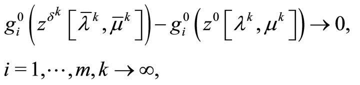
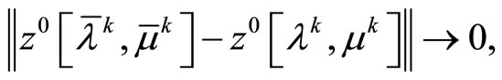
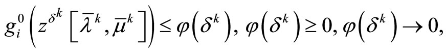
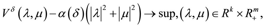
Theorem 4.3. Assume that the set D is bounded and is a continuous convex functional. For a minimizing approximate solution to problem (P⁰) to exist (and, hence, every its weak limit point belongs to Z^*), it is necessary and sufficient that there exists a sequence of dual variables

,

such that

,

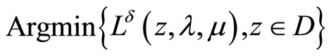
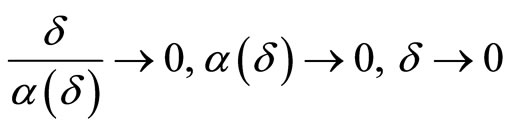
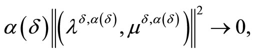
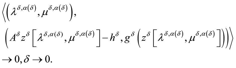
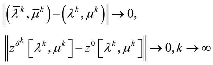
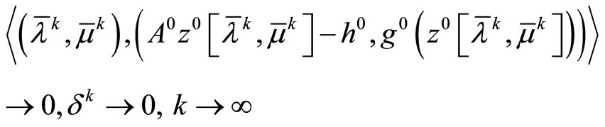
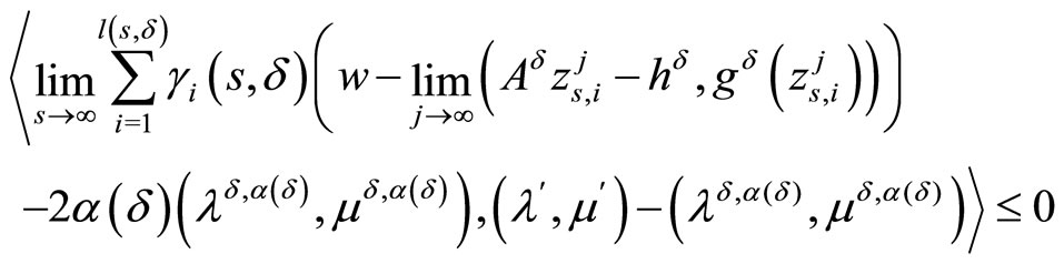
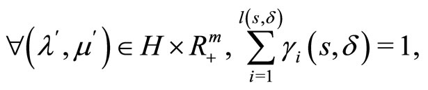
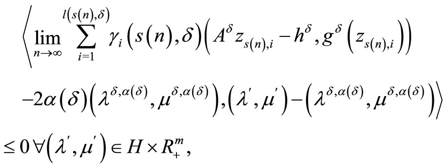
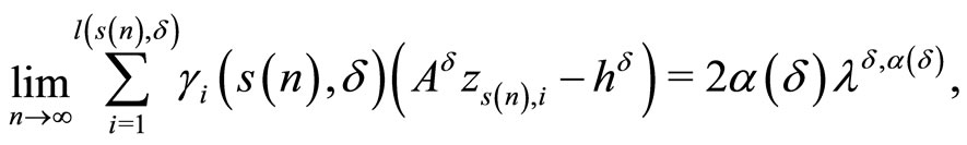
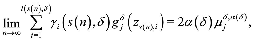
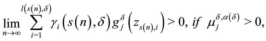
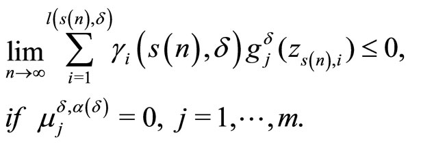
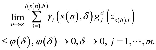
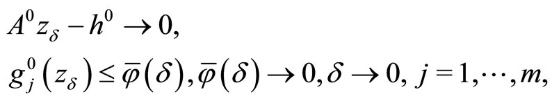
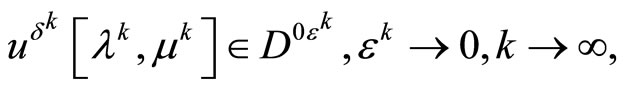
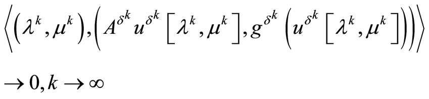
and the relations

(29)

(30)

hold for some elements

.

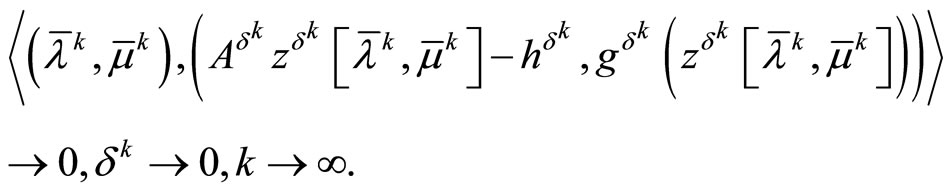
Moreover, the sequence

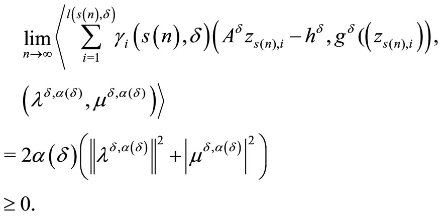
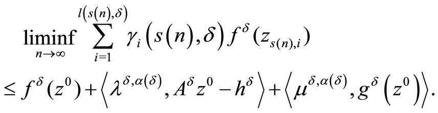
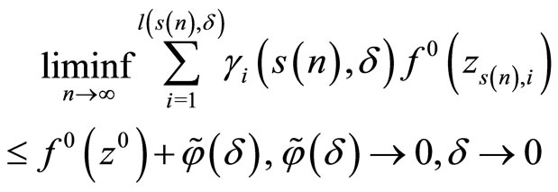
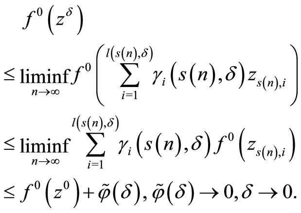
is the desired minimizing approximate solution, and every weak limit point of this sequence is a solution to Problem (P⁰). As a consequence of the limit relations (29), (30) the limit relation

(31)

holds. Simultaneously, every weak limit point of the sequence

is a maximizer of the dual problem

.

Proof. To prove the necessity, we first observe that Problem (P⁰) is solvable, i.e., because of the conditions on its input data and existence of minimizing approximate solutions. Now, the first two limit relations (29), (30) of the present theorem follow from Theorem 3.3. if and are chosen as the points

,

and respectively. Further, due to the estimate (19) and the limit relation

,

we have

Then, taking into account the equality (see (23))

the limit relation (30) and obtained limit relation

(see (22)) we can write

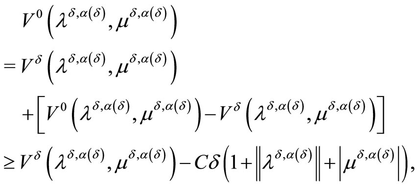
and, as consequence, the limit relation (31) is valid. So, we have shown that the limit relation (31) is a consequence of the limit relations (29), (30). Now, let the sequence

be bounded. Then, since the concave continuous functional V⁰ is weakly upper semicontinuous, every weak limit point of this sequence is a maximizer of the dual problem.

Now we prove the sufficiency. We first observe that the set

is nonempty in view of the inclusion

the boundedness of the sequence

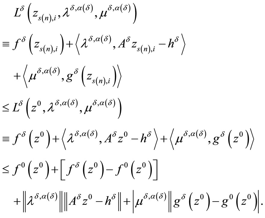
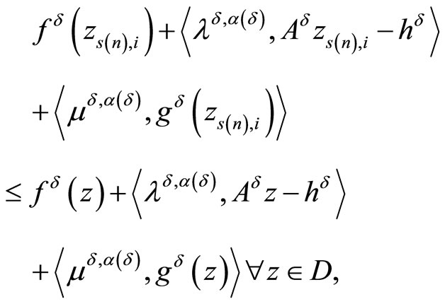
and the conditions imposed on the initial data of Problem (P⁰). Hence, problem (P⁰) is solvable. Furthermore, since the point is a minimizer of the Lagrange functional, we can write

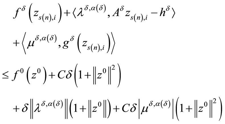
By the hypotheses of the theorem, this implies that

We set in this inequality and use the consistency condition

,

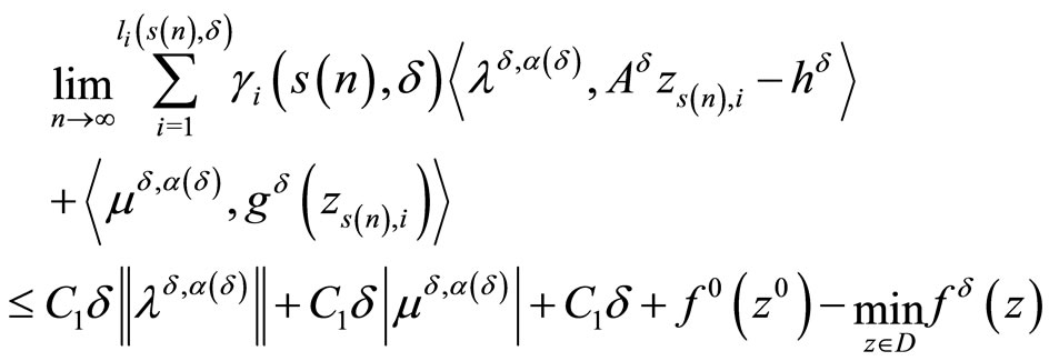
to obtain

,.

In addition we have

.

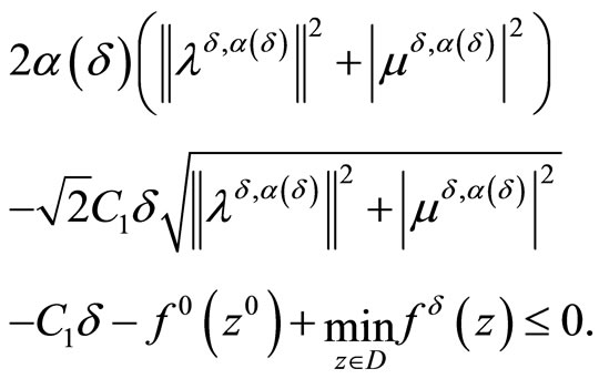
Using the classical properties of the weak compactness of a convex closed bounded set and the weak lower semicontinuity of a convex continuous functional, we easily deduce from the above facts that

i.e. the sequence

is a minimizing approximate solution of Problem (P⁰).

5. Possible Applications of the Stable Sequential Kuhn-Tucker Theorem

Below in this section we consider two illustrative examples connected with possible applications of the results obtained in the previous sections. Its main purpose is to show principal possibilities of using various variants of the stable sequential Kuhn-Tucker theorem for solving optimal control and inverse problems.

5.1. Application in Optimal Control

First of all we consider the optimal control problem with fixed time and with functional equality and inequality constraints

Here and below, is a number characterising an error of initial data, is a fixed number,

is a convex functional,

are convex functionals,

,

are Lebesgue measurable and uniformly bounded with respect to matrices,

are Lebesgue measurable and uniformly bounded with respect to vectors,

,

is a convex compact set, is a solution to the Cauchy problem

Obviously, for each control this Cauchy problem has a unique solution and all these solutions are uniformly bounded with respect to and

(32)

Assume that

whence we obtain due to the estimate (32) for some constant

Define the Lagrange functional

and the concave dual functional

Define also the notations

Here and below, we leave the notation accepting in Section 1.

Let             

denote the unique point in that maximizes on this set the functional

Applying in this situation, for example in the case of convexity of, Theorem 4.3 we obtain the following result.

Theorem 5.1. For a minimizing approximate solution to Problem to exist (and, hence, every its weak limit point belongs to), it is necessary and sufficient that there exists a sequence of dual variables

,

such that

    ,

and the relations

(33)

(34)

hold for some elements

.

Moreover, the sequence

is the desired minimizing approximate solution, and every weak limit point of this sequence is a solution to Problem. As a consequence of the limit relations (33), (34) the limit relation

holds. Simultaneously, every limit point of the sequence

is a maximizer of the dual problem

.

The points, may be chosen as the points, where,.

In conclusion of this subsection, we note that the Pontryagin maximum principle can be used for finding optimal elements in the problem

(35)

Denote

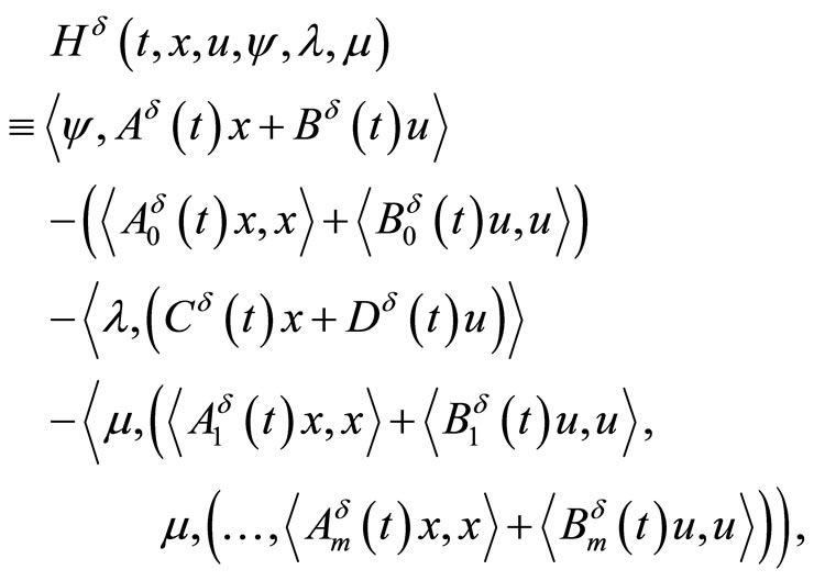
where is matrix with lines , is matrix with lines.

Then, due to convexity of the problem (35) we can assert that any its minimizer satisfies the following maximum principle.

Theorem 5.2. The maximum relation

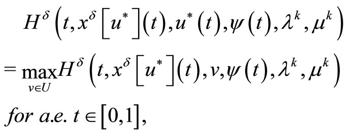
holds for the Lagrange multipliers, where, is the solution of the adjoint problem

5.2. Application in Ill-Posed Inverse Problems

Now we consider the illustrative example of the ill-posed inverse problem of final observation for a linear parabolic equation in the divergent form for recovering a distributed right-hand side of the equation, initial function, and boundary function on the side surface of the cylindrical domain for the third boundary value problem. Here we study the simplified inverse problem with a view of compact presentation. Similar but more general inverse problem may be found in [10].

Let, and be convex compacts,

,

,

be a bounded domain in, ,

,

,

.

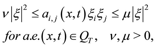
Let us consider inverse problem of finding a triple of unknown distributed, initial, and boundary coefficients for the third boundary value problem for the following linear parabolic equation of the divergent form

(36)

determined by a final observation

whose value is known approximately, at a certain. Here, similar to [11],

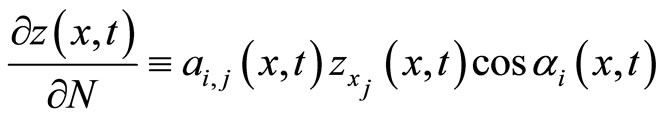
and is the angle between the external normal to and the axis, and is a number characterising an error of initial data, is a fixed number. The solution to the boundary value problem (36) corresponding to the desired actions is a weak solution in the sense of the class [11]. Clearly, the solution to the inverse problem in such a statement may be not unique. Therefore, we will be interested in finding a normal solution, i.e., a solution with the minimal norm

which we denote by.

It is easy to see that the above-formulated inverse problem of finding the normal solution by a given observation is equivalent to the following fixed-time optimal control problem on finding a minimum-norm control triple with strongly convex objective functional and a semi-state equality constraint

      

where

The input data for the inverse problem (and, hence, for Problem are assumed to meet the following conditions:

1)       functions

,

are Lebesgue measurable;

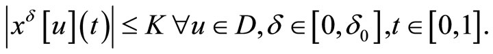
2)       the estimates

hold, where K > 0 is a constant not depending on;

3)       the boundary S is piece-wise smooth.

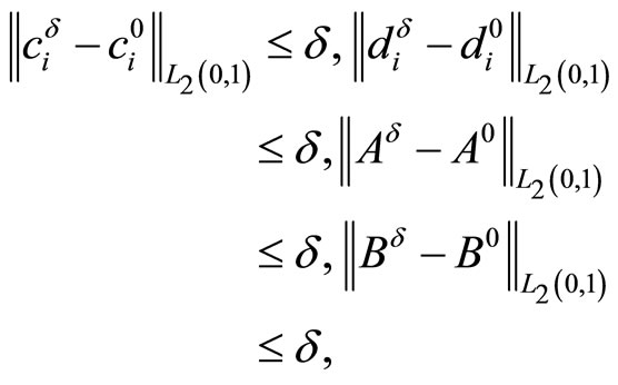
Denote by approximate final observation (with parameter) and assume that

(37)

From conditions 1) - 3) and the theorem on the existence of a weak (generalized) solution of the third boundary value problem for a linear parabolic equation of the divergent type [11], (Chapter III, Section 5), [12] it follows that the direct problem (36) is uniquely solvable in for any triple and any T > 0 and besides a priory estimate

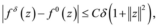
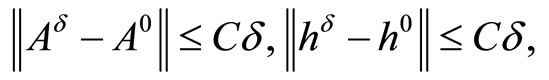
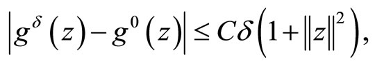
is true, where a constant C > 0 not depends on. The last facts together with the estimates (37) lead to corresponding necessary estimate for deviation of perturbed linear bounded operator,

from its unperturbed analog (details may be found in [10])

where a constant C > 0 not depends on.

Define the Lagrange functional

with the minimizer and the concave dual functional

Let denotes the unique point in that maximizes on this set the functional

Applying Theorem 4.1. in this situation of strong convexity of we obtain the following result.

Theorem 5.3. For a bounded minimizing approximate solution to Problem to exist (and, hence, to converge strongly to as), it is necessary that there exists a sequence of dual variable, , such that, , the limit relations

(38)

are fulfilled. Moreover, the latter sequence is the desired minimizing approximate solution to Problem; that is,

.

At the same time, the limit relation

(39)

is fulfilled.

Conversely, for a minimizing approximate solution to problem to exist, it is sufficient that there exists a sequence of dual variable, such that

, the limit relations (38) are fulfilled. Moreover, the latter sequence is the desired to Problem; that is,

.

Besides, the limit relation (39) is also valid. Simultaneously, every weak limit point of the sequence, is a maximizer of the dual problem

.

The points, may be chosen as the points

, where,.

Since the set D is bounded in Problem, we can apply for solving our inverse problem the regularized Kuhn-Tucker theorem in a form of iterated process also. Thus, Theorem 4.2. leads us to the following theorem.

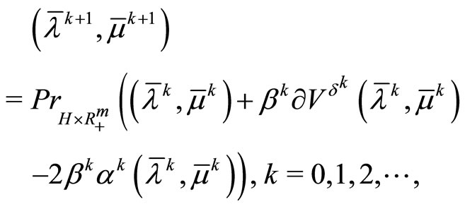
Theorem 5.4. For a minimizing approximate solution to Problem to exist (and, hence, to converge strongly to), it is necessary that for the sequence of dual variable, , generated by iterated process

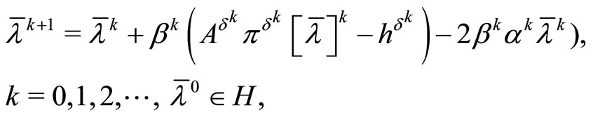(40)

with the consistency conditions (8) the limit relations

(41)

are fulfilled. In this case the sequence

is the desired minimizing approximate solution to Problem; that is,

.

Simultaneously, the limit relation

(42)

is fulfilled.

Conversely, for a minimizing approximate solution to Problem to exist, it is sufficient that for the sequence of dual variable, , generated by iterated process (40) with the consistency conditions (8), the limit relations (41) are fulfilled. Moreover, the sequence

is the desired minimizing approximate solution to Problem; that is,

.

Simultaneously, the limit relation (42) is valid.

REFERENCES

NOTES

^*This work was supported by the Russian Foundation for Basic Research (project no. 12-01-00199-a) and by grant of the Ministry of Education and Science of the Russian Federation (project no. 1.1907.2011)

REFERENCES

- V. M. Alekseev, V. M. Tikhomirov and S. V. Fomin, “Optimal Control,” Nauka, Moscow, 1979.
- F. P. Vasil’ev, “Optimization Methods,” Faktorial Press, Moscow, 2002.
- M. Minoux, “Mathematical Programming. Theory and Algorithms,” Wiley, New York, 1986.
- M. I. Sumin, “Duality-Based Regularization in a Linear Convex Mathematical Programming Problem,” Journal of Computational Mathematics and Mathematical Physics, Vol. 47, No. 4, 2007, pp. 579-600. doi:10.1134/S0965542507040045
- M. I. Sumin, “Ill-Posed Problems and Solution Methods. Materials to Lectures for Students of Older Years. TextBook,” Lobachevskii State University of Nizhnii Novgorod, Nizhnii Novgorod, 2009.
- M. I. Sumin, “Parametric Dual Regularization in a Linear-Convex Mathematical Programming,” In: R. F. Linton and T. B. Carrol, Jr., Eds., Computational Optimization: New Research Developments, Nova Science Publishers Inc., New-York, 2010, pp. 265-311.
- M. I. Sumin, “Regularized Parametric Kuhn-Tucker Theorem in a Hilbert Space,” Journal of Computational Mathematics and Mathematical Physics, Vol. 51, No. 9, 2011, pp. 1489-1509. doi:10.1134/S0965542511090156
- J. Warga, “Optimal Control of Differential and Functional Equations,” Academic Press, New York, 1972.
- A. N. Tikhonov and V. Ya Arsenin, “Methods of Solution of Ill-Posed Problems,” Halsted, New York, 1977.
- M. I. Sumin, “A Regularized Gradient Dual Method for Solving Inverse Problem of Final Observation for a Parabolic Equation,” Journal of Computational Mathematics and Mathematical Physics, Vol. 44, No. 12, 2004, pp. 1903-1921.
- O. A. Ladyzhenskaya, V. A. Solonnikov and N. N. Ural’tseva, “Linear and Quasilinear Equations of Parabolic Type,” Nauka, Moscow, 1967.
- V. I. Plotnikov, “Uniqueness and Existence Theorems and a Priori Properties of Generalized Solutions,” Doklady Akademii Nauk SSSR, Vol. 165, No. 1, 1965, pp. 33-35.