Theoretical Economics Letters
Vol.2 No.5(2012), Article ID:25811,5 pages DOI:10.4236/tel.2012.25090
A Microeconomic Foundation for the Phillips Curve under Complete Markets without any Exogenous Price Stickiness: A Keynesian View
1Institute of Social Science, University of Tokyo, Tokyo, Japan 2Department of Economics, Kanagawa University, Yokohama, Japan
Email: ohtaki@iss.u-tokyo.ac.jp, tamai-y@kanagawa-u.ac.jp
Received June 23, 2012; revised July 25, 2012; accepted August 28, 2012
Keywords: Long-Run Downward-Sloping Phillips Curve without Any Price Stickiness Assumption; Intergenerational Learning Effect; Negative Correlation between Labor Productivity and Inflation Rate
ABSTRACT
Assuming that labor productivity varies with the previous employment level, we derive the Phillips curve based on the standard dynamic microeconomic foundation. The usage of the term standard implies that our theory entirely excludes assumptions unfamiliar to microeconomics such as price or information stickiness, and money in the utility function. We find that when labor productivity decreases, disinflation advances. This is because disinflation, ceteris paribus, limits the current goods supply and increases the rate of return on money (the inverse of the inflation rate) in an overlapping generations (OLG) model. In addition, mass unemployment becomes a hazard for the intergenerational skill transformation, and thus, the higher the unemployment is, the lower the labor productivity becomes in the stationary state. Consequently, the negative correlation between inflation and unemployment emerges even in the dynamic general equilibrium in complete markets. It is also noteworthy that we depend neither on linear approximations nor on numerical methods: the method used to derive the Phillips curve is purely analytical.
1. Introduction
Every work on the Phillips curve presumes some market imperfection. For example, Lucas [1] assumes that the equilibrium price is a noisy signal disturbed by monetary shocks. Calvo [2] and Woodford [3] stochastically confine the opportunity of price realignment. Mankiw and Reis [4] insist that there exist some substantial diffusive lags that inform the necessity of price revision. These works imply that if there does not exist some price stickiness assumption or imperfect information (that is, the markets are complete), the negative correlation between inflation and unemployment will disappear, and the vertical Phillips curve will reemerge as Friedman [5] suggests. This also means that money is neutral in the long run, when all adjustments are complete.
Our main concern in this article is to establish with certainty the stationary negative correlation between inflation and unemployment without price frictions. Doing so would not only enable us to interpret the Phillips curve as the long-run trade-off relationship as in the original work (Phillips [6]) but also contribute toward shortening the gulf between macroeconomic and microeconomic theory.
The change in labor productivity due to the learning effect plays a crucial role in this paper. Although recent works addressing the Phillips curve have focused on the responses of inflation and unemployment to a monetary shock, the effect of a real shock (namely, the change in the labor productivity rate) should also be seriously considered. Hayashi and Prescott [7] reveal that significant declines in the total factor productivity (TFP) and hours worked were observed in Japan during the 1990s. It is also noteworthy that disinflation was prominent throughout that decade, despite the easy monetary policy.
The decline in the labor productivity, which partially consists of the TFP, results in disinflation in the deterministic overlapping generations (OLG) model of Otaki [8,9], even if we do not make any price-stickiness assumptions a priori. When labor productivity is lowered, ceteris paribus, the current goods supply is reduced, and this increases the rate of return on money (the inverse of the inflation rate). Thus, the decline in labor productivity is accompanied by disinflation1.
We further assume that skills nurtured through production process is transmitted to the child generation, and that more the employment opportunities offered to fathers, the more productive children become. This relationship is assumed to be based on the increase in educational opportunities from the income growth, and, perhaps unintentionally, educational effect within a family. In brief, the current labor productivity is assumed to be an increasing function of the previous employment level.
In stationary states, in which the employment level is kept constant, the fewer the employment level is, the fewer the productive individuals. Consequently, there emerges a negative correlation between inflation and the unemployment rate. This is our understanding of the long-run Phillips curve or the aggregate supply curve under complete markets.
The paper is organized as follows. Section 2 exhibits the basic model. The Phillips curve is also derived. Section 3 addresses with the economic welfare implications of the expansionary fiscal-monetary policy. Section 4 contains brief concluding remarks.
2. Model
2.1. Model Structure
We consider a standard two-period OLG model. There exist continuous individuals  who supply labor at their discretion only when they are young. Each firm monopolistically produces the differentiated good that is distributed within [0,1]. The monopoly rent is equally distributed among the young regardless of their employment status.
Fiat money is the only store of value. The government finances its expenditure by seigniorage. For simplicity, we assume that the goods purchased by the government bear no additional utility to the individuals.
2.2. Individuals
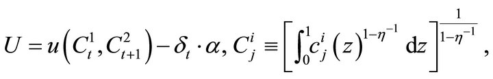
Each individual maximizes the following lifetime utility function:
 (1)
(1)
where  denotes the consumption of good
  by the individuals in the
  th stage of life during period
 .
. ![]() is the disutility of labor, and
is the disutility of labor, and  is a definition function that takes the values one (when employed) and zero (when unemployed). In addition, we assume that
 ![]() is a linear homogenous function.
is a linear homogenous function.
Then, the indirect utility function  of
of ![]() is represented as
is represented as
 (2)
(2)
where  is the nominal wage and
  is the aggregate nominal monopoly rent. We must note that
  is also linear homogenous.
Using (2), we can calculate the nominal reservation wage  as
as
 (3)
(3)
Since our main concern is the imperfect employment equilibrium in which some individuals are always unemployed and possess no bargaining power,  becomes the equilibrium nominal wage2.
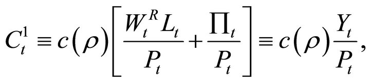
It is also noteworthy that the following aggregate consumption function of the younger generation  is obtained from the linear homogeneity of
![]() :
:
 (4)
(4)
where

denotes the gross inflation rate.  is the aggregate employment level.
2.3. Firms
From (1), each firm faces the following aggregate demand function :
:
 (5)
(5)
where  is the aggregate employment level. Furthermore, we assume that each firm
  has the following production function
 :
:
 (6)
(6)
 is the function of the productivity of labor, which plays a key role in our comparative statics. (6) implies that there is a socially significant learning effect in the productivity of labor. That is, when the fewer individuals of the previous generation are employed (the unemployment rate
  becomes higher) and fewer skills for production are socially accumulated, the more difficult is to transmitted these skills to the current generation3.
The profit maximization problem leads to the following optimal pricing rule:
 (7)
(7)
Aggregating (7) on , we obtain the following important difference equation:
 (8)
(8)
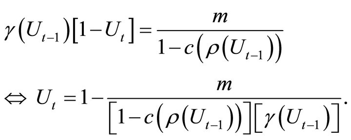
From the linear homogeneity of , Equation (8) determines the equilibrium inflation rate
  independently of the nominal money supply. Differentiating (8) logarithmically and using Roy’s identity, we obtain
 (9)
(9)
where ![]() is the elasticity of the labor productivity to the unemployment level. The left-hand side of Equation (9) indicates the number of future goods that can be substituted for present goods when inflation occurs.
is the elasticity of the labor productivity to the unemployment level. The left-hand side of Equation (9) indicates the number of future goods that can be substituted for present goods when inflation occurs.
From Equation (9), it is clear that the inflation rate  is determined so as to equalize the additional present aggregate supply reduction
to the additional savings
 .
.
That is, a disimprovement in the labor productivity implies a potential decrease in the current consumption level; this suppresses inflation and increaces the rate of return on money to promote savings.
2.4. Government
In this model, the role of the government is very simple. It issues new money,  , to finance wasteful expenditure
 . Avoiding any diversion from the stationary equilibrium, we assume that the expenditure is controlled so as to keep the real money stock
 , constant over time. Hence, the budget constraint of the government can be written as
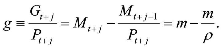 (10)
(10)
2.5. Market Equilibrium
2.5.1. The Aggregate Demand Function
Since our attention is confined to the imperfect employment equilibrium, the labor markets are in equilibrium whenever . The real aggregate demand
  is defined as
 (11)
(11)
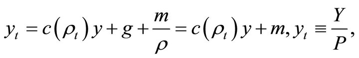
where the third term of Equation (11) is the consumption demand of the old individuals and the government expenditure. This is the dynamically extended multiplier process developed by Otaki [8,9]. Solving Equation (11), we obtain
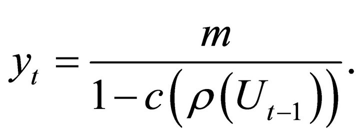 (12)
(12)
Equation (12) is the aggregate demand function of our model. It can be easily seen that an expansionary fiscal-monetary policy increases the real GDP as long as the inflation rate is kept constant.
2.5.2. The Long-Run Phillips Curve
We have already established the negative correlation between inflation and unemployment in 2.3. The Phillips curve is implicitly defined by Equation (9). Consequently, the Phillips curve is obtained as illustrated by Curve  in Figure 1.
2.5.3. Market Equilibrium
The goods market equilibrium is expressed by the solution of (8) and (12). Since the aggregate production function is defined by
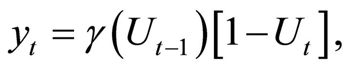 (13)
(13)
substituting this equation into the aggregate demand function (12), we obtain the equilibrium condition for the aggregate goods market as
 (14)
(14)
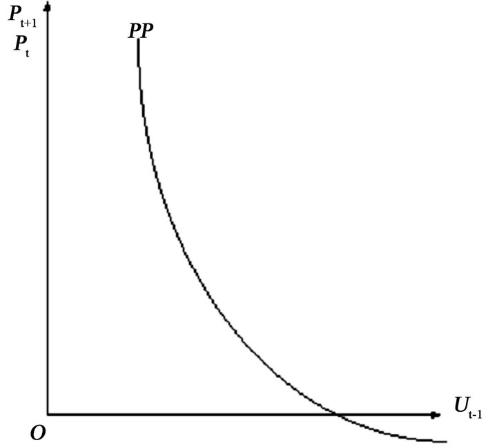
Figure 1. Phillips curve.
It is clear that the right-hand side of (14) is an increasing function of  as long as
This implies that the intertemporal substitution rate on consumption is positive and the rise of the unemployment rate,  , is not too high. From empirical analyses4, it does not seem so restrictive an assumption.
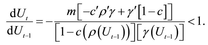
In such a case, the locus of (14)  is upward sloping as illustrated by Figure 2. It is apparent from the Figure that a sufficient stability condition of the stationary state
  is that Curve
  cuts a
  line from above; thus, we assume that the stationary state is stable5.
The fiscal-monetary policy shifts the location of Curve  downward as in Figure 2. That is, fiscal-monetary expansion results in a decrease in the unemployment rate. This implies that a discretionary expansion in the fiscalmonetary policy can increase the real GDP
 ![]() together with accelerating inflation and labor productivity.
together with accelerating inflation and labor productivity.
3. The Welfare Implication of Fiscal-Monetary Policy
Since the indirect lifetime utility is represented by Equation (2), considering that the labor supply is never in surplus, the social welfare  is defined as
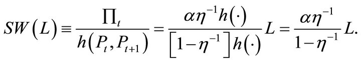 (15)
(15)
Let us analyze the welfare implication of our macroeconomic policy in the imperfect employment equilibrium. The result can be easily obtained from Figure 2 and Equation (15). From Figure 2, it is apparent that the real money supply ![]() increases the real GDP
increases the real GDP ![]() and employment level
and employment level![]() . Accordingly, Equation (15) reveals that the social welfare is always enhanced by an expansionary fiscal-monetary policy.
. Accordingly, Equation (15) reveals that the social welfare is always enhanced by an expansionary fiscal-monetary policy.
4. Concluding Remarks
We have developed the microeconomic foundation for the Phillips curve under complete markets. The obtained
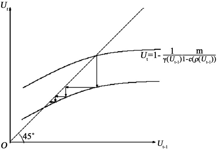
Figure 2. The dynamics of the labor market.
results are as follows.
First, the Phillips curve can be derived not from a monetary shock but from an endogenous structure of the economy per se. Whenever the labor productivity increases, inflation rises because the current consumption needs to be stimulated in accordance with the potential increase in production capacity. Hence, the rate of return on money decreases, and the inflation rate increases. Thus, a positive correlation between the labor productivity and inflation emerges.
On the other hand, lower labor productivity is reproduced by itself. That is, mass unemployment of the previous generation deprives the current generation of the formal and informal educational opportunities. Thus, the lower employment level causes lower labor productivity, and a stationary negative correlation between inflation and unemployment emerges, even under complete markets.
Second, as long as the stationary state is stable, an expansionary policy can raise the real GDP and improve social welfare. This is because the expansionary policy increases the real GDP by the multiplier process and improves labor productivity through reduction of the unemployment level.
REFERENCES
- R. E. Lucas Jr., “Expectations and the Neutrality of Money,” Journal of Economic Theory, Vol. 4, No. 2, 1972, pp. 103-124. doi:10.1016/0022-0531(72)90142-1
- G. A. Calvo, “Staggered Prices in a Utility-Maximizing Framework,” Journal of Monetary Economics, Vol. 12, No. 3, 1983, pp. 383-398. doi:10.1016/0304-3932(83)90060-0
- M. Woodford, “Control of the Public Debt: A Requirement for Price Stability?” NBER Working Papers, 1996.
- N. G. Mankiw and R. Reis, “Sticky Information versus Sticky Prices: A Proposal to Replace the New Keynesian Phillips Curve,” Quarterly Journal of Economics, Vol. 117, No. 4, 2002, pp. 1295-1328. doi:10.1162/003355302320935034
- M. Friedman, “The Role of Monetary Policy,” American Economic Review, Vol. 58, No. 1, 1968, pp. 1-17.
- A. W. Phillips, “The Relation between Unemployment and the Rate of Change of Money Wage Rates in the United Kingdom, 1861-1957,” Economica, Vol. 25, No. 100, 1958, pp. 283-299.
- F. Hayashi and E. C. Prescott, “The 1990s in Japan: A Lost Decade,” Review of Economic Dynamics, Vol. 5, No. 1, 2002, pp. 206-235. doi:10.1006/redy.2001.0149
- M. Otaki, “The Dynamically Extended Keynesian Cross and the Welfare-Improving Fiscal Policy,” Economics Letters, Vol. 96, No. 1, 2007, pp. 23-29. doi:10.1016/j.econlet.2006.12.005
- M. Otaki, “A Welfare Economics Foundation for the FullEmployment Policy,” Economics Letters, Vol. 102, No. 1, 2009, pp. 1-3. doi:10.1016/j.econlet.2008.08.003
- I. M. McDonald and R. M. Solow, “Wage Bargaining and Employment,” American Economic Review, Vol. 71, No. 5, 1981, pp. 896-908.
- K. J. Arrow, “The Economic Implications of Learning by Doing,” Review of Economic Studies, Vol. 29, No. 3, 1962, pp. 155-173. doi:10.2307/2295952
- L. P. Hansen and K. J. Singleton, “Stochastic Consumption, Risk Aversion, and the Temporal Behavior of Asset Returns,” Journal of Political Economy, Vol. 91, No. 2, 1983, pp. 249-265. doi:10.1086/261141
- J. Y. Campbell and N. G. Mankiw, “Consumption, Income, and Interest Rates: Reinterpreting the Time Series Evidence,” NBER Macroeconomics Annual, Vol. 4, 1989, pp. 185-216. doi:10.2307/3584973
NOTES
1The same mechanism—intertemporal substitution—is also adopted by Lucas [1].
2However, the nominal wage might exceed the reservation wage when the individuals possess collective bargaining power. Nevertheless, as long as the nominal wage negotiation is efficient in the sense of McDonald and Solow [10], there is no need to discuss any modification. See Otaki [9] for the precise proof.
3This is an overlapping-generations model version of Arrow’s [11] learning by doing. Unemployment generally makes the education for the next generation more difficult because of the reduction in incomes. These unhappily educated children also possibly affect some negative effects to their school as a whole, although, needless to say, there are many exceptional students who overcome such difficult circumstances.
4For example, see Hansen and Singleton [12] and Campbell and Mankiw [13].
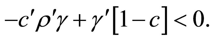
5The stability condition requires
It is clear above inequality that whenever the real money supply m is sufficiently small, the dynamics of the economy is stable. Unless such condition is satisfied, the economy autonomously attains the full-employment equilibrium or degenerates into the zero employment equilibrium depending on where the economy is initially located. Both cases seems quite unnatural in reality, and hence we assume the economy is stable.