Theoretical Economics Letters
Vol. 2 No. 1 (2012) , Article ID: 17373 , 4 pages DOI:10.4236/tel.2012.21014
On Transportation Cost and Product Differentiation in Hotelling’s Model
School of Business, East China University of Science and Technology, Shanghai, China
Email: liyouping@ecust.edu.cn
Received October 8, 2011; revised November 15, 2011; accepted November 24, 2011
Keywords: Hotelling’s model; transportation cost; product differentiation
ABSTRACT
We model transportation cost in Hotelling’s model as a general exponential function and analyze firms’ location choice. As a first step, we take prices as exogenous and focus on the positioning strategy of the firm whose product generates a lower net-of-price utility. We find the firm locates further away from its competitor when the transportation cost (if convex) becomes more convex and when it (if concave) becomes more concave. Minimum differentiation is obtained when the transportation cost is linear in travel distance.
1. Introduction
Linear and quadratic forms of transportation cost have been widely used in spatial competition models [1,2]. The main reason for social scientists’ preference towards these functional forms is their mathematical solvability. However, there is little justification, theoretically or empirically, to rule out the possibility of a concave transportation cost. As was noted by Thisse and Vives [3], in the geographical context typically, because of scale economies in transportation, transportation cost is a concave function of distance. This is the case especially when the cost of time is also considered. Very likely, the time spent on shopping, for example, is an increasing function on travel distance but at a decreasing rate.1 In a more general sense, the disutility from choosing the product with a characteristic different from one’s most preferred taste can take either form.
In this paper, we model a consumer’ transportation cost in Hotelling’s model as a general exponential function, thus incorporating both the convex and concave cases. As a first step, we take prices as exogenous and focus on the positioning strategy of the firm whose product generates a lower net-of-price utility level (the lessfavored firm). This simplification has been frequently applied to public choice models [4] (referred to as the Hotelling-Downs model). In political elections, the candidates have different valence characters which are known to the public. But they do have some flexibility in choosing a political stance (or policy) in the campaign. The application of the model in industrial economics is somehow limited, as only in a few settings prices charged by a firm is not a choice variable. One example is, franchised stores in a local market whose prices are set by their national franchisors only have store location as a choice variable.
The rest of the paper is organized as follows. In Section 2, we set up the model and study the less-favored firm’s location strategies. In Section 3, we run a simple numerical simulation to illustrate the results obtained in Section 2. In Section 4, we conclude this paper and discuss future work.
2. The Model
Consider two firms supplying a homogenous product in a market represented by the Hotelling line . They have the same constant marginal cost which is normalized to zero. Consumers are uniformly distributed along the market and have unit demand. Let
  denote Firm i’s location,
 . For a consumer at
 , the utility derived from buying product from Firm i is
where the parameter  is the utility derived from consuming the product of Firm i (net of the price paid). The second part in the utility function is transportation cost which is an exponential function of travel distance, with
 . This general form of transportation cost incorporates the linear case (
 ) and the quadratic case (
 ) used in the literature. When
  , transportation cost is concave in travel distance. We normalize b to one to simplify notation.
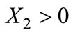
Without loss of generality, assume  . For instance, Firm 1 charges a lower price than Firm 2 for some reason, or it has a better reputation and consumers derive higher utility from doing business with Firm 1. If firms simultaneously choose a location, or Firm 1 chooses a location after Firm 2, the problem becomes trivial: Firm 1 may simply locate at the same spot as Firm 2 and Firm 2 earns zero profit.2 As a result, we focus on the case of a sequential play with Firm 2 being the second mover and we assume Firm 1’s location is exogenous.3 This captures at least some interesting scenarios. For example, in industrial economics, Firm 2 is the entrant into a market where Firm 1 had been the monopolist. In the political elections, then Firm 2 represents the challenger to a position held by Firm 1, the incumbent whose political position has been well known. Assume Firm 1 locates at
 .
.
Define  as the difference in utilities from buying the two firms’ products to a consumer locating at x:

This consumer chooses to buy from Firm 2 if  .4 After observing Firm 1’s location choice,
  , Firm 1’s objective is to choose a location
  such that
  is positive for the widest range of consumers. With
 , Firm 2 would choose
  . To avoid the trivial solution that Firm 1 takes the whole market regardless of Firm 2’s choice, we assume the following condition is satisfied:
 .
.
Let 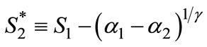 be the location at which if Firm 2 locates there the consumer at the same location is indifferent between the two firms. That is,
 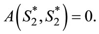 Then we have (All proofs are in the Appendix):
Proposition 1: If ,
,  , and consumers within the range
 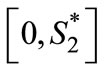 buy the product from Firm 2.
If ,
,  , and consumers within the range
  buy the product from Firm 2, where
 is the solution to
 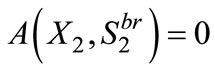 .
.
The positioning strategy for the less-favored firm is quite different in the two cases. Figure A1 and Figure A3 in the Appendix A illustrate the reason: at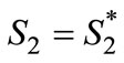 , Firm 2’s advantage,
  , increases as a consumer locates further to the left from that point when the transportation cost is convex (
 ), but it decreases (and becomes negative) when the transportation cost is concave (
 ). As a result, when
 , Firm 2 should choose
 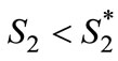 to ensure that
  is positive for at least some consumers.
However, this does not mean that product differentiation would be higher when , since the value of
  also changes with
 . The following proposition can be proved:
Proposition 2: When , the greater
  is, the closer to Firm 1 Firm 2 chooses to locate. When
 , the greater
  is, the further away from Firm 1 Firm 2 chooses to locate. Minimum differentiation occurs when
 .
.
Thus the functional form of transportation cost in Hotelling’s model plays an important role in determining the magnitude of product differentiation. This has not received much attention in previous studies. In the next section, we will illustrate the result using some numerical examples.
3. Numerical Examples
As we have noted, the more-favored firm, Firm 1, would locate at the center if it could make such a choice before Firm 2 moves. Figure 1 shows the best response strategies for Firm 2 when 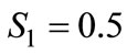 and
and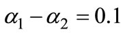 . As we can see, Firm 2 locates the closest to Firm 1 at
  when
when . It moves further away from its competitor as the transportation cost becomes more convex or more concave.
Figure 2 is another example showing Firm 2’s location choices when Firm 1 is not at the center. For example, a right-wing incumbent is constrained from changing his conservative view in a political election. As we can see, a similar result is obtained. In this case, the lessfavored firm may earn a larger market share (winning an election) if the transportation cost is not too concave or too convex ( close to 1).
Figure 1. Firm 2’s location choice (S1 = 0.5).
Figure 2. Firm 2’s location choice (S1 = 0.7).
4. Conclusions
In this note, we generalize the functional form of transportation cost in Hotelling’s model to incorporate both the convex and concave cases. As we have shown, the positioning strategy of the less-favored firm is quite different under the two cases and minimum differentiation occurs when the transportation cost is linear in travel distance.
As a first step, we assumed that location is the only choice variable in the competition. This is suitable for models of political election; however, it has limited power in explaining horizontal differentiation in industrial economics when product price is also at the firms’ discretion. Considering both the pricing and positioning strategies under the more general form of transportation cost may be challenging but also meaningful for future researches.
REFERENCES
- H. Hotelling, “Stability in Competition,” Economic Journal, Vol. 39, No. 153, 1929, pp. 41-57. doi:10.2307/2224214
- C. D’Aspremont, J. J. Gabszewicz and J.-F. Thisse, “On Hotelling’s ‘Stability in Competition’,” Econometrica, Vol. 47, No. 5, 1979, pp. 1145-1150.
- J.-F. Thisse, and X. Vives, “On the Strategic Choice of Spatial Price Policy,” American Economic Review, Vol. 78, No. 1, 1988, pp. 122-137.
- A. Downs, “An Economic Theory of Democracy,” Harper and Brothers, New York, 1957.
- S. Ansolabehere and J. M., Snyder, “Valence Politics and Equilibrium in Spatial Election Models,” Public Choice, Vol. 103, No. 3-4, 2000, pp. 327-336. doi:10.1023/A:1005020606153
- M. Dix and R. Santore, “Candidate Ability and Platform Choice,” Economics Letters, Vol. 76, No. 2, 2002, pp. 189-194. doi:10.1016/S0165-1765(02)00047-2
Appendix A
Proof of Proposition 1
The first part is easily shown by the monotonicities of 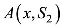 with respect to x for the ranges
 ,
,  and
and  respectively (See Figure A1 and Figure A2 for an illustration).
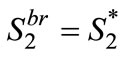
However, this does not apply to the case when  (See Figure A3).
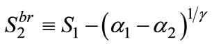
Actually, Firm 2 should choose  to ensure that
  is positive for at least some consumers. For any choice of
  by monotonicities of
  , there are only two solutions to
  ,
,  and
and , with
  and
and . Firm 2 sells to consumers in the range
  if
if , or
, or  if
if . Also, we have
which means Firm 2 should move as far away from Firm 2 as possible to enlarge the range . However, consumers reside only in
 . So Firm 2 should choose a location such that
  (See Figure A4).
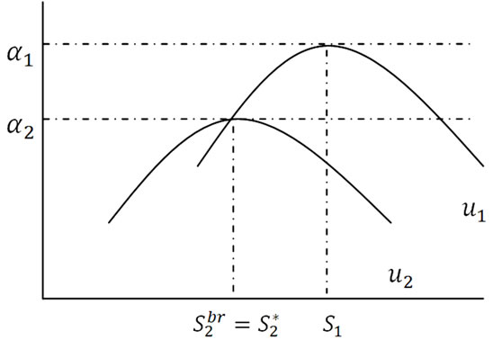
Figure A1. Consumer utilities (γ > 1).
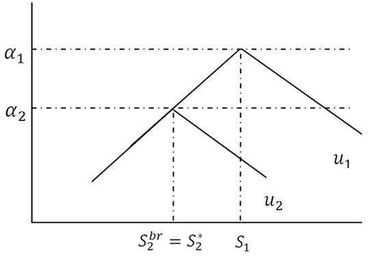
Figure A2. Consumer utilities (γ = 1).
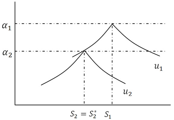
Figure A3. Consumer utilities (0 < γ < 1).

Figure A4. Consumer utilities (0 < γ < 1).
Solving 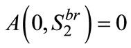 , we get the Firm 2’s optimal location choice:
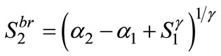 . ■
. ■
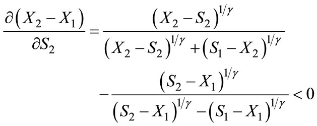
Proof of Proposition 2
When ,
,  , which is strictly decreasing in
 . When
 ,
,  , which is strictly increasing in
 . Thus we only need to show that
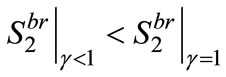 . From the above formula, we have
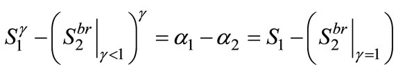 . Notice that the function
  is strictly increasing in
  for
for  and
and . Suppose
 then
then 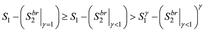 a contradiction. ■
NOTES
1For a longer distance, a consumer may be able to drive on a highway and save on time (and gasoline as well).
2That firms locate at a same spot may not be an equilibrium or may not be a unique equilibrium. For more discussions, see, e.g., Ansolabehere and Snyder [5] and Dix and Santore [6], both assuming quadratic trasportation costs.
3Firm 1 would choose locating at the middle, S1 = 0.5, if it were to make a choice. What we derive in the following is more general.
4We make the condition only weakly positive to simplify discussion. Note that if the consumer randomizes its purchase when A(x,S2) = 0, a best response strategy for Firm 2 does not exist when γ = 1.