American Journal of Operations Research
Vol. 3 No. 1A (2013) , Article ID: 27558 , 10 pages DOI:10.4236/ajor.2013.31A020
An Intelligent Control Technique for Dynamic Optimization of Temperature during Fruit Storage Process
Department of Biomechanical Systems, Ehime University, Matsuyama, Japan
Email: morimoto@agr.ehime-u.ac.jp
Received October 31, 2012; revised November 30, 2012; accepted December 15, 2012
Keywords: Dynamic Optimization; Fruit-Storage Temperature; Water Loss; Neural Networks; Genetic Algorithms
ABSTRACT
Agricultural control systems are characterized by complexity and uncertainly. A skilled grower can deal well with crops based on his own intuition and experience. In this study, an intelligent optimization technique mimicking the simple thinking process of a skilled grower is proposed and then applied to dynamic optimization of temperature that minimizes the water loss in fruit during storage. It is supposed that the simple thinking process of a skilled grower consists of two steps: 1) “learning and modeling” through experience and 2) “selection and decision of an optimal value” through simulation of a mental model built in his brain by the learning. An intelligent control technique proposed here consists of a decision system and a feedback control system. In the decision system, the dynamic change in the rate of water loss as affected by temperature was first identified and modeled using neural networks (“learning and modeling”), and then the optimal value (l-step set points) of temperature that minimized the rate of water loss was searched for through simulation of the identified neural-network model using genetic algorithms (“selection and decision”). The control process for 8 days was divided into 8 steps. Two types of optimal values, a single heat stress application, such as 40˚C, 15˚C, 15˚C, 15˚C, 15˚C, 15˚C, 15˚C and 15˚C, and a double heat stress application, such as 40˚C, 15˚C, 40˚C, 15˚C, 15˚C, 15˚C, 15˚C and 15˚C, were obtained under the range of 15˚C £ T £ 40˚C. These results suggest that application of heat stress to fruit is effective in maintaining freshness of fruit during storage.
1. Introduction
Storage temperature for fruits is usually maintained constant at low level. This is because the low temperature effectively reduces microbial spoilage and water loss of the fruit. In recent years, however, there has been much interest in heat treatments that reduce the quality loss of fruit during storage [1,2]. It has been reported that heat treatment is effective for inhibiting ethylene production and delaying the ripening [3-7], for controlling insect pests and for reducing chilling injury [4,8] of fruit. It has been also reported that heat treatment can improve fruit quality [9-11].
It is known that the exposure of living organisms to heat stress produces several types of heat shock proteins (HSPs) in their cells, which acquire transient thermal tolerance [12,13]. Recently, the relationships between the heat treatment and HSPs have been investigated to elucidate the effects of heat treatment [14]. Acquiring thermo tolerance may lead to the reduction of water loss for fruits during storage [15]. It is, therefore, important to know how to apply the heat stress to the fruit in order to minimize loss of quality. A dynamic optimization technique will give us the solution.
It is, however, very difficult to treat and realize optimization control of water loss of fruits during storage when we take the response of thermo tolerance caused by heat stress into consideration. This is because the physiological behaviors between the temperature and the water loss of the fruit, including the effect of thermo tolerance, are quite complex and uncertain. They are characterized by strong non-linearity and time-variation.
A skilled grower can deal well with complex systems such as many types of crops during cultivation and fruits during storage using his own intuition and experience. In order to realize the optimization control of complex systems such as agricultural production processes, therefore, it seems very useful to imitate the thinking process of a skilled grower [16,17].
It is well known that intelligent approaches such as neural networks and searching technique using genetic algorithms are effective tools for imitating the skilled grower’s thinking process. Neural networks mimic the human learning process and can identify nonlinear relationships between inputs and outputs of a system with their own high learning abilities [18]. Genetic algorithms mimic the biological evolutionary process and search for an optimal value in parallel with a multi-point search procedure, based on crossover and mutation in genetics [19,20]. An intelligent control technique combining neural networks with genetic algorithms has been developed for realizing the optimization of cultivation and storage processes [16,17,21]. It is also thought that the problem of time-variation of the physiological status of the fruit is possible to solve by repeating identification (learning) and modeling of the input and output system.
In this study, an intelligent optimization technique mimicking a skilled grower’s simple thinking process is proposed and then applied to find the variable temperature profile (l-step set points of temperature) of the storage chamber to minimize water losses of tomatoes. With this technique, neural networks and genetic algorithms are successfully employed for mimicking the “learning and modeling” and “selection and decision” of a skilled grower.
2. Speaking Fruit Approach (SFA) for Dynamic Optimization Control
Storage temperature for fruit is usually maintained constant at a low level, already determined as an optimal value, without any consideration of the physiological status of the fruit. In order to achieve the qualitative improvement of the fruit, however, it is essential to control the environment flexibly and optimally, taking the physiological status of the fruit into consideration. Measurement of the fruit responses and control based on the fruit’s physiological information are major tasks for realizing the optimization of the storage process. The storage environment should be controlled optimally based on fruit responses. This approach is called a “speaking fruit” approach (SFA) [22]. Figure 1 shows a schematic diagram of a computer control system for fruit and vegetables during storage under the SFA concept. The control system consists of several sensors to measure
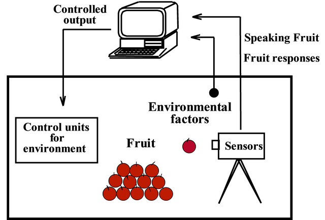
Figure 1. The concept of a “speaking fruit approach (SFA)”.
the physiological responses of the fruit, a computer to determine the optimal set points of the environment, and control devices to control the environment based on the optimal set points. Non-destructive measurements of fruit responses are essential for realizing dynamic optimization control. Thus, in this study, the dynamic optimization control is carried out based on the fruit responses, aiming at the qualitative improvement of the fruit during storage.
3. Optimization Problem
Tomatoes (Solanum lycopersicum L. Momotaro) were used for the experiment. Freshness is one of the most important evaluation factors that consumers use to select tomatoes at market. In order to maintain the freshness of tomatoes during storage, the storage temperature is usually maintained constant at a lower level. In recent years, however, it has been reported that a heat stress application is also effective for maintaining the quality of tomato [9-11]. This is probably due to thermo tolerance of the fruit acquired by heat stress. The aim for optimization in this study is to minimize the rate of water loss of tomato during storage by optimal control of the temperature.
Let WT(k) (k = 1, 2, ···, N) be a time series of the rate of water loss, as affected by temperature T(k) at time k. An objective function, F(T), is given by the average value of the rate of water loss during the last period  of the control process.
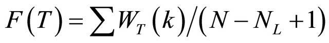 (1)
(1)
where NL and N are the first and last time points, respectively, in the evaluation period.
Note that the rate of water loss was evaluated at the last period  in the control process. This is because the influence of heat stress is thought to appear at the latter half stage if heat stress was applied to the fruit during the first period of the control process.
For realizing optimization, the control process was divided into 8 steps, because the length of the control process was 8 days. Therefore, the optimization problem here is to determine the 8-step set points of the temperature, which minimize the objective function F(T). That is, an optimal value is given by the optimal combination of the 8-step set points for temperature (Top1, ···, Top8). As for the constraint of the temperature, we had two minimum temperatures (5˚C as a normal temperature for a refrigerator, and 15˚C as an average temperature for shelf life in Japan) in order to investigate the influence of the heat stress at adequate temperature levels. As for the maximum temperature, 40˚C was determined to be best for heat stress from previous literature [1-3] and from considerations for a one-day application of heat stress.
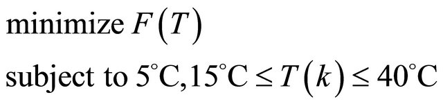 (2)
(2)
4. Measuring Systems
Mature green tomatoes of uniform size (about 8 cm in diameter) were stored in a storage chamber (Tabai-espec, LHU-112M), where the temperature and relative humidity are strictly controlled by a personal computer with an accuracy of ±0.1˚C and ±2% RH, respectively. Three tomatoes were used for each experiment. The rate of water loss of the tomato was estimated from the weight loss. The weight loss of the tomato was continuously measured by hanging a cage containing three tomatoes using an electronic balance (Sartorius, LP-620S). In this case, the electronic balance was set outside of the chamber in order to remove the effect of the temperature change. The relative humidity was maintained constant at 60% ± 2% RH while only the temperature was flexibly changed based on a system control manner. The sampling time was 10 min.
5. Design of a Control System
5.1. A Skilled Grower’s Thinking Process
A skilled grower can deal well with crops based on his own intuition and experience. Figure 2 shows the conceptual diagram of a simple thinking process for his cultivation strategy. It mainly consists of two steps. The first step is a “learning and modeling” process. A grower first cultivates a crop by trial and error over several years and learns the growth behaviors of the crop from experience. This is the process of making a mental model of crop growth in his brain through learning. The second step is a “simulation (or prediction) and decision” process for selecting the best cultivation method. A grower predicts and simulates the crop growth using the mental model built in his brain and selects the best strategy for the next cultivation from among many results obtained by simulation. After a decision, a grower takes an action for the best strategy.
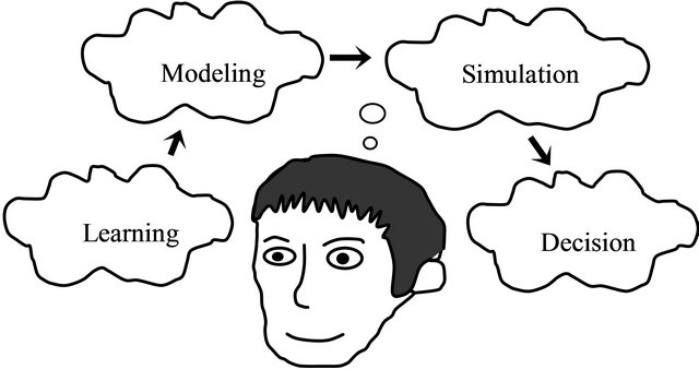
Figure 2. Conceptual diagram of a decision procedure of a skilled grower on the basis of his simple thinking process.
5.2. An Intelligent Control System for Dynamic Optimization
The procedure shown in Figure 2 can be realized by introducing neural networks and genetic algorithms. Figure 3 shows the block diagram of an intelligent control system mimicking a simple thinking process of a skilled grower, which is applied for realizing the optimization control of the rate of water loss [16,17,21]. It consists of a decision system and a feedback control system. The decision system, consisting of neural networks and genetic algorithms, determines the optimal set point trajectory of the temperature. In the decision system, the rate of water loss, as affected by temperature, is first identified using the neural network, and then the optimal combination of the l-step set points of the temperature that minimize the objective function is searched for through simulation of the identified neural-network model using the genetic algorithm. The diagrammatical view of this simulation method is shown in Figure 5.
It is found that this control technique including neural networks and genetic algorithms well reflects a human thinking process. The first action, identification and modeling, using neural networks, are similar to the manner in which a skilled grower makes a mental model in his brain through learning or experience (learning). In the second step, the way to obtain an optimal value corresponds to the procedure by which a skilled grower selects a better (or best) strategy from his own experience and prediction (decision).
It will be found that if these two procedures, identification and the search for an optimal value, are repeated periodically during the storage process to adapt to the time variation of the physiological status of the fruit, then both optimization and adaptation can be satisfied.
5.3. Neural Network Application for Identification
Neural networks are used for identifying the dynamic
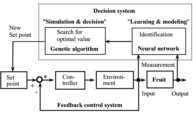
Figure 3. An intelligent control system for realizing the optimal control of the storage process based on the SFA concept.
response of the rate of water loss as affected by the temperature and for creating a black-box model for simulation. Figure 4 shows a time-delay neural network used for dynamic identification. It consists of three layers and has arbitrary feedback loops that produce time histories of the data for dynamic identification [23]. The input variable is the temperature, T(k), and the output variable is the rate of water loss, WT(k). The well-known timedelay neural-network model is given as [24]:
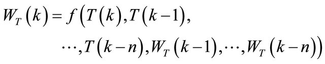 (3)
(3)
where n is the system order (system parameter number). The unknown function f(×) can be approximated by the neural network.
For the learning of the neural network, the (n+1)th historical input data 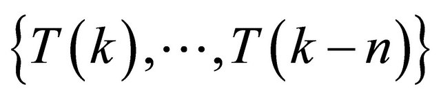 and the nth historical output data
  are applied to the input layer, and the current output,
  , is applied to the output layer as a training signal
  data number). The learning (training) method is error back-propagation [25]. It tunes weights and biases of the neural network so that the squared error between the network output and the training signal is minimized. Through these procedures, a dynamic model is obtained.
For prediction, the current output,  , is estimated from both the (n + 1)th past historical input data
  and the nth past historical output data
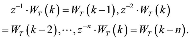
  like an ARMA model procedure [23,26]. The time series of
are obtained by applying backward shift operators  to the variable WT(k) through the following procedures:
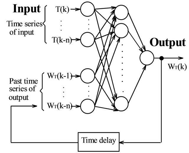
Figure 4. Structure of a three-layer neural network with time-delay operator.
The data for identification are divided into two data sets, a training data set and a testing data set. The former is used for training the neural network, and the latter is used for evaluating the accuracy of the identified model. The testing data sets have to be independent of the training data sets.
The most important task for determining the model’s structure is the choice of the system parameter number. Here, the system parameter number and the hidden neuron number of the neural-network were determined based on the cross-validation [27].
5.4. Genetic Algorithm Application for Searching for an Optimal Value
Here, genetic algorithms are used for searching for the optimal 8-step set points of the temperature that minimize the objective function through model simulation. Figure 5 shows a diagrammatical view of this simulation method. The total combination number of the input (8- step stet points of temperature) under the constraint of 15˚C to 40˚C was 268 sets because we took the increment of 1˚C between 15˚C and 40˚C in each step. Therefore, numerous output responses of the rate of water loss are obtained through simulation.
In order to use genetic algorithms, an “individual” for evolution should be defined as the first step. Each individual represents a candidate for an optimal value. Since an optimal value to be obtained here is the 8-step set points of temperature, an individual can be given by the 8-step set points of temperature . They were all coded as 6-bit binary strings, which gives numerical values between 0 (000000) and 63 (111111).
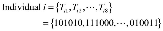
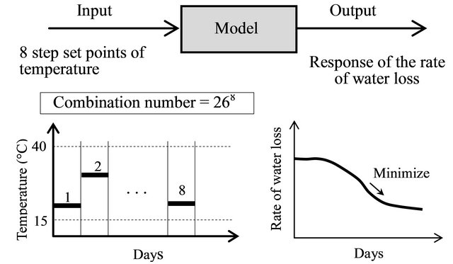
Figure 5. A method for finding an optimal value (combination of the 8-step set points) of the temperature that minimizes the rate of water loss through simulation.
A set of individuals is called a “population”. They evolve toward better solutions. Genetic algorithms work with a population involving many individuals.
Fitness is an indicator for measuring an individual’s survival quality. All individuals are evaluated by their fitness values. During the evolution process, therefore, individuals having higher fitness reproduce, and individuals with lower fitness die in each generation. An individual having the maximum fitness is regarded as an optimal solution. Fitness is similar to the objective function. So, fitness can be represented by Equation (1).
 (4)
(4)
The crossover operation is a single crossover. Two individuals (e.g., 000011 and 101111) are first mated at random. These binary strings are cut at the 3-bit position along the strings and then two new individuals (000111 and 101011) are obtained by swapping all binary characters from the 1-bit to the 3-bit position. The mutation inverts one or more components of the binary strings, selected at random from the population, from 0 to 1 or vice versa. Here, a two point mutation was used. One individual (e.g., 101111) is first selected at random, and then a new individual (001011) is created by inverting two characters, selected at random, from 0 to 1 or 1 to 0. The mutation operation increases the variability of the population and helps to avoid the possibility of falling into local optima [28]. The selection of individuals was carried out based on the elitist strategy by which an individual with maximum fitness is compulsorily remained for next generation. However, the operation’s searching performance can easily fall into a local optimum because only the superior individuals with higher fitness are picked in each generation. In this study, therefore, different individuals in another population were added into the original population in order to maintain the diversity.
Figure 6 shows the flow chart of the genetic algorithm. The procedure is as follows. (Step 1): The initial population consisting of Ni (=6) types of individuals is generated at random. (Step 2): No (=100) types of individuals are added to the original population from another population in order to maintain the diversity of the original population. (Step 3): Genetic operations, crossover and mutation, are applied to those individuals. Through the crossover, Nc sorts of individuals are newly created according to the crossover rate , and Nm sorts of individuals are then newly generated according to the mutation rate
 . From these operations,
  types of individuals are obtained. (Step 4): The fitness (values of the objective function) of all individuals are calculated using the neural-network model, and their performances are evaluated. (Step 5): Superior individuals,
  individuals with higher fitness, are selected and retained for the next
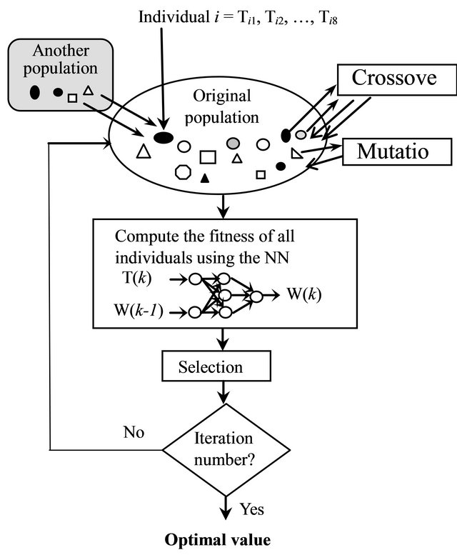
Figure 6. Flow chart of the genetic algorithm used for searching for an optimal value.
generation based on elitist strategy selection. (Step 6): Steps 2 to 5 are repeated until the fitness continues to keep the same minimum value with increasing generation number. An optimal value is given by an individual with minimum fitness.
6. Dynamic Responses of the Rate of Water Loss to Temperature
Figure 7 shows a typical dynamic response of the rate of water loss as affected by the up and down of temperature. The temperature was first increased from 25˚C to 35˚C to 40˚C and then decreased from 40˚C to 35˚C to 25˚C. The rate of water loss of the fruit increased in proportion with temperature. However, comparing to the two values of the rate of water loss at the same temperature, before increasing and after dropping the temperature, it is found that the values after dropping the temperature are lower than those before increasing the temperature at both the 25˚C and 35˚C conditions. These results suggest that a temperature operation that first rises to the high level (35˚C to 40˚C) and then drops to the prior level has a tendency to reduce the rate of water loss, as compared to when the temperature was maintained constant throughout the control process. This is probably due to the effect of thermo tolerance of the fruit caused by high temperature stress. It is, therefore, difficult to identify and model the water loss of the fruit as affected by temperature using a conventional mathematical equation.
The data for identification were obtained. Figure 8
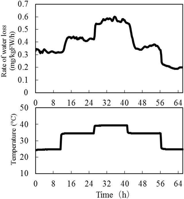
Figure 7. A dynamic response of the rate of the water loss, as affected by the temperature.
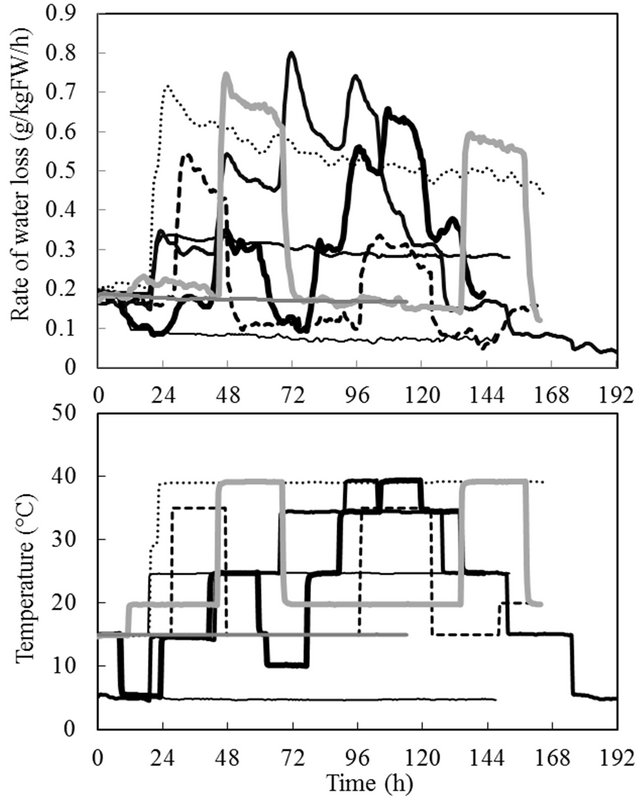
Figure 8. Typical dynamic changes in the rate of the water loss, as affected by temperature (8 patterns).
shows typical eight types of dynamic changes in the rate of water loss as affected by temperature for about 192 h. Here, 13 types of date sets on the controlled input and output were obtained. Among them, twelve data sets were used for training and one data set was used for validation of the neural network. The temperature was flexibly changed between 5˚C and 40˚C to identify clearly the dynamics of the rate of water loss as affected by temperature. Short-term heat stresses of 40˚C for about 24 h were included in several temperature operations. From the figure, it is found that, in all cases, the rate of water loss dynamically changes with the temperature.
7. Identification Result of the Rate of Water Loss to Temperature
The system parameter number and the hidden neuron number of the neural network were determined based on the cross-validation. Figure 9 shows the relationship between the system parameter number n and the estimated error in the identification. It is found that the estimated errors for the 15th system parameter number gave a minimum error. Through these considerations, the system parameter number n and the hidden neurons nh were determined to be 15 and 20, respectively.
Figure 10 shows the comparison of the estimated response, calculated from the neural network model, and the observed response for the rate of water loss. A testing data set, which is quite different from the training data sets, was used for this comparison. It was found that the estimated response was very closely related to the observed response. Significant decreases in the rate of water loss after dropping the temperature from higher levels to lower levels, which are thought to be caused by thermo tolerance, observed in the model response of 60 to 120 h. That is, the values of the rate of water loss after dropping the temperature from 40 ® 35 at 96 h and 35˚C ® 27˚C at 108 h are lower than those before increasing the temperature from 35 ® 40 at 84 h and 27˚C ® 35˚C at 72 h, respectively. These results mean that the neuralnetwork model could acquire such complex response as a thermo tolerance, and we succeeded in making a suitable model for searching for an optimal value.
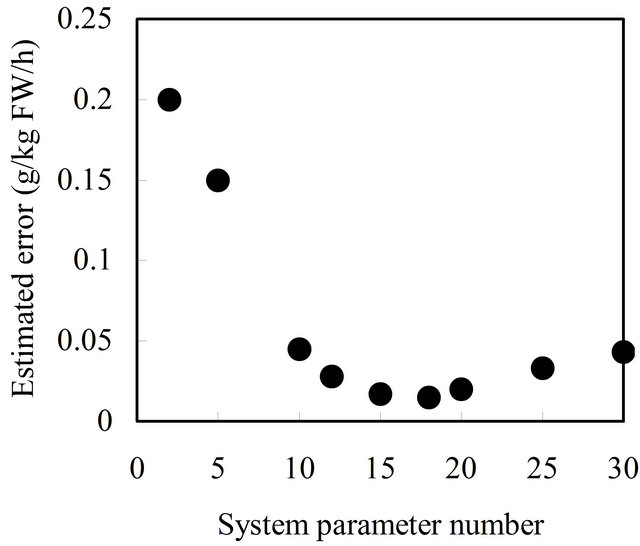
Figure 9. Relationship between the system parameter number n and the estimated error.
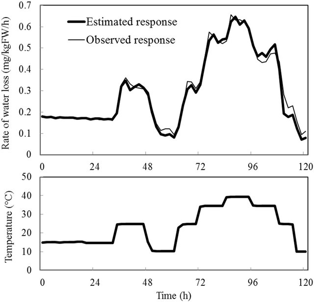
Figure 10. Comparison of the estimated and observed responses of the rate of the water loss.
Figure 11 shows the estimated relationship between the temperature and the rate of water loss of a tomato, calculated from the simulation of the identified neuralnetwork model. Open squares represent real observed data. It is found that the estimated values are closely related to the observed values. The rate of water loss increases with temperature. In the range over 35˚C, it has a tendency to decrease with temperature. This means that the water loss was significantly suppressed by high temperature. It is also found that the relationship between temperature and the rate of water loss is non-linear.
8. The Search for an Optimal Value Through Model Simulation
Next, the optimal combination of the 8-step set points for temperature was searched for through simulation of the identified neural-network model using the genetic algorithm. Figure 12 shows the evolution curves in searching for an optimal under the different crossover and mutation rates. The horizontal axis is the generation number for evolution and the vertical axis is the fitness of the best individual in each generation. The fitness dramatically decreased with generation number, and then lowered down to the minimum value. The search was stopped when the fitness continued to keep the same minimum value, and that individual was considered to give the minimum fitness as an optimal value.
It was found that the convergence speed was larger for the higher crossover and mutation rates (Pc = 0.8 and Pm = 0.6) than for the lower crossover and mutation rates (Pc = 0.1 and Pm = 0.01). The fitness could not decrease to the minimum value and fell into a local optimum when
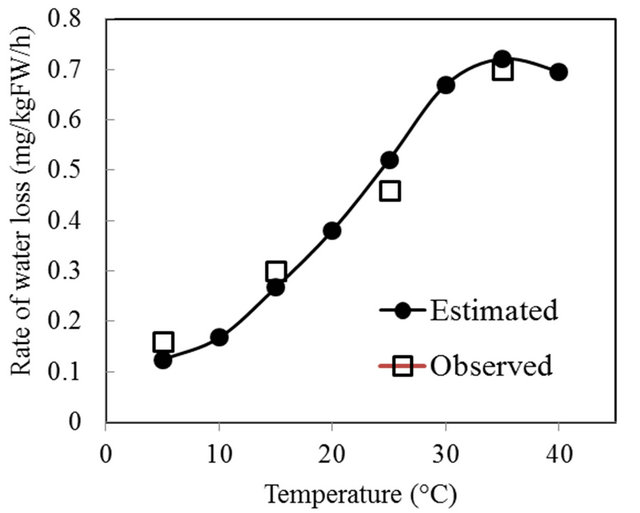
Figure 11. The static relationship between the temperature and the rate of the water loss, obtained from simulation of the identified model.

Figure 12. An evolution curve in searching for an optimal value when the evaluation length is the latter half stage of the control process (96 to 192 h).
the crossover and mutation rates decreased to lower values. The searching performance usually depends on the diversity of the population [16]. A global optimal value could be obtained if the diversity in the population was maintained at a high level in each generation. Higher crossover and mutation rates were shown to be effective in keeping a higher diversity in the population, but excessively high crossover and mutation rates are time consuming. The values of Pc = 0.8 and Pm = 0.6, which were determined through a trial and error, were enough high to avoid a local optimum.
There is no guarantee that genetic algorithms yield a global optimal solution. It is, therefore, important to confirm whether an optimal value determined by genetic algorithm is global or local. In this paper, the confirmation was mainly carried out using a round-robin algorithm, which systematically searches for all possible solutions around the optimal solution at the proper step. This is because a near global optimal solution can at least be obtained by genetic algorithms. An optimal solution was confirmed with a different initial population and different methods of crossover and mutation.
Through these investigations, several types of optimal values were obtained under different constraints of the temperature. When the constraint was 5˚C £ Tl £ 40˚C, two optimal values, a combination of only the lowest temperature Tl = {5˚C, 5˚C, 5˚C, 5˚C, 5˚C, 5˚C, 5˚C, 5˚C} and a combination of heat stress and the lowest temperature Tl = {40˚C, 5˚C, 5˚C, 5˚C, 5˚C, 5˚C, 5˚C, 5˚C}, were selected. There was no significant difference in the rate of water loss between the two operations after the heat stress. This is because, under a low temperature, these two responses were very small; consequently, it was difficult to compare their values.
Next, therefore, we increased the minimum temperature level and defined the constraint as 15˚C £ Tl £ 40˚C in order to extract the effect of the heat stress. In this constraint, we had two optimal values under the different evaluation lengths of the control process. For example, when the evaluation length was the latter half stage (96 – 216 h) of the control process, a single heat stress application of 40˚C during the first 24 h, Tl = {40˚C, 15˚C, 15˚C, 15˚C, 15˚C, 15˚C, 15˚C, 15˚C} was found to be an optimal value. The length of each step is 24 h. A double heat stress application, Ti = {40˚C, 15˚C, 40˚C, 15˚C, 15˚C, 15˚C, 15˚C, 15˚C}, was also found to be an optimal value when the evaluation length was restricted to only the last two steps (168 – 216 h) of the control process. Two optimal values (single and double heat stresses) were characterized by the combination of the highest temperature (40˚C) and the lowest temperature (15˚C).
9. Optimal Control Performances
Finally, the optimal values for single and double heat stresses obtained were applied to a real storage system. Figure 13 shows an optimal control performance of the rate of water loss when a single heat stress (Tl =40˚C, 15˚C, 15˚C, 15˚C, 15˚C, 15˚C, 15˚C, 15˚C) was applied to the fruit. Here, the responses of the water loss obtained by integrating the rate of water loss are also shown in the figure in order to compare their total amount of water loss. The bold line shows the case of optimal control, and the fine line shows the case of a constant-temperature TL = {15˚C, 15˚C, 15˚C, 15˚C, 15˚C, 15˚C, 15˚C, 15˚C}. The initial temperature was kept at 15˚C for 24 h, and then the optimal control started. The 8-day control process from 24 to 216 h was divided into eight steps. In this case, the evaluation length is the latter half step of the control process (96 – 216 h = 5 days), and the constraint of the temperature is 15˚C £ T £ 40˚C. It is found that, after the single heat stress application, the rate of water loss became lower in the optimal control than in the constantvalue control.
Figure 14 shows an optimal control performance of the rate of water loss when double heat stresses (Tl = 40˚C, 15˚C, 40˚C, 15˚C, 15˚C, 15˚C, 15˚C, 15˚C) was applied to the fruit. The bold line shows the case of the optimal control, and the fine line shows the case of a constant-temperature (Tl = {15˚C, 15˚C, 15˚C, 15˚C, 15˚C, 15˚C, 15˚C, 15˚C}). The evaluation length was only the last two steps of the control process (168 – 216 h = 2 days), and the constraint was 15˚C £ T £ 40˚C. The initial temperature was kept at 15˚C for 24 h, and then the optimal control started.
From the optimal control performance, the rate of water loss after the second heat stress (double heat stress) is lower than that after the first heat stress (single heat stress). Thus, the rate of water loss had a tendency to decrease after each application of the heat stress. After the double heat stresses, therefore, the value becomes much lower than that in the constant-value control. However, the degree of the reduction caused by the heat stress
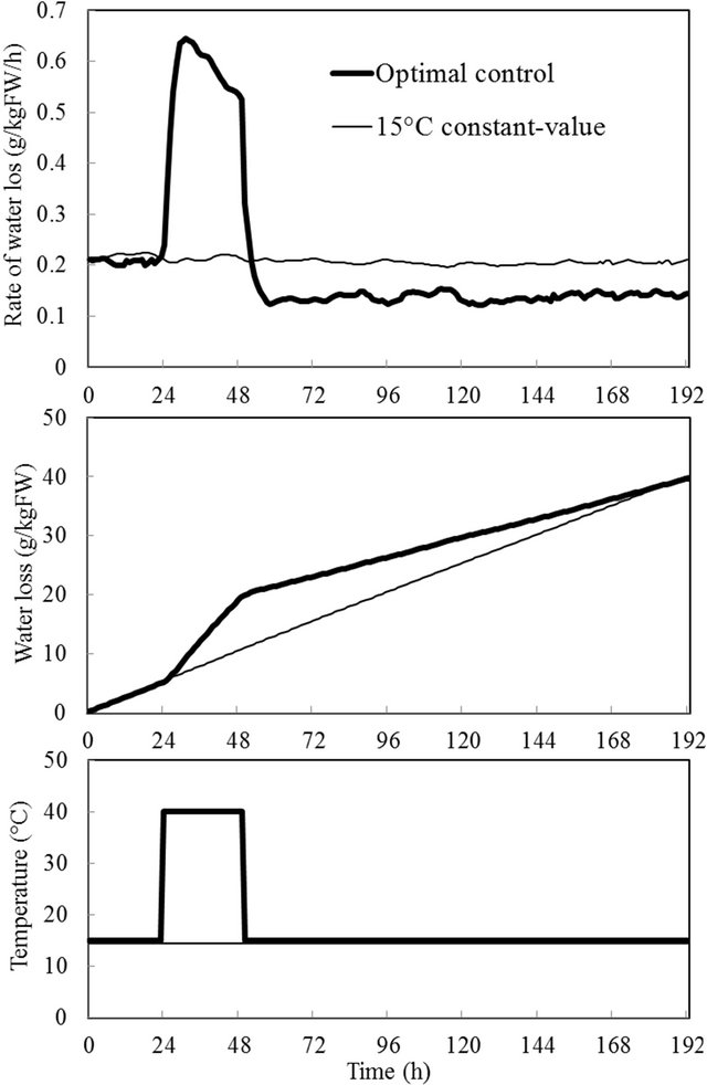
Figure 13. An optimal control performance of the rate of the water loss as affected by the single heat stress when the evaluation length is the latter half stage of the control proc ess (96 to 192 h) under the temperature range (15˚C £ T(k) £ 40˚C).
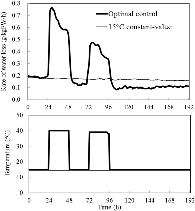
Figure 14. An optimal control performance of the rate of the water loss as affected by the double heat stress when the evaluation length is only last two steps of the control process (144 to 192 h) under the temperature range (15˚C £ T(k) £ 40˚C).
decreases with the application number of the heat stress. In addition, the values of the rate of water loss during the second heat stress application were much lower than that during the first heat stress application. This is because the first heat stress significantly suppressed the water loss of the fruit. It was confirmed that this significant reduction after the second heat stress application continues for at least 3 or 4 more days from other experiments.
In this study, we focused on the rate of water loss, not the total amount of water loss, in order to apply a dynamic control for optimization. This is because the rate of water loss, against the temperature, is more sensible and controllable than the amount of the water loss. It is also clear that since the total amount of water loss is obtained by integrating the rate of water loss, the response speed is always slow.
The reduction of the water stress caused by the heat stress suggests that the heat-stress fruits acquired a transient thermo tolerance. Controlling temperature so that it first rises to the highest level and then drops to the lowest level seems to be especially effective at reducing the water loss of the fruit during storage, as compared with 15˚C-constant control. This means that the optimal applications of the heat stress to a low temperature operation is more effective than only a low temperature operation in order to reduce the water loss of fruit during storage. It is also suggested that the physiological responses of the fruit can be improved by applying heat stress optimally to the fruit. This is a marked characteristic of a living thing. In any cases, a control method that changes flexibly and optimally on the basis of fruit responses is useful to improve fruit quality during storage.
10. Conclusions
In this study, the optimal 8-step set points of the temperature that minimize the rate of water loss of the fruit during storage was determined using neural networks and genetic algorithms. The length of each step is 24 h. Under the range of 15˚C £ T £ 40˚C, two types of optimal operations, a single heat stress operation {40˚C, 15˚C, 15˚C, 15˚C, 15˚C, 15˚C, 15˚C, 15˚C} and a double heat stress operation {40˚C, 15˚C, 40˚C, 15˚C, 15˚C, 15˚C, 15˚C, 15˚C}, were obtained for different evaluation lengths of the control process. These are characterized by the combinations of the highest temperature (40˚C) and the lowest temperature (15˚C). It is especially emphasized that the sudden drop of the temperature from the highest level (40˚C) to the lowest level (15˚C) had a tendency to decrease the water loss of the fruit compared to when the temperature was maintained at the lowest level. The reduction of the water stress caused by the heat stress suggests that the heat-stress fruits acquired a transient thermo tolerance. These results suggest that a control method that applies the 40˚C - 50˚C heat stress to the fruit optimally on the basis of fruit responses is a better way to maintain fruit quality during storage than a conventional control manner that simply maintains the temperature at the lowest level.
REFERENCES
- S. Lurie, “Review Postharvest Heat Treatments,” Postharvest Biology and Technology, Vol. 14, No. 3, 1998, pp. 257-269.
- L. B. Ferguson, S. Ben-Yehoshua, E. J. Mitcham, R. E. McDonald and S. Lurie, “Postharvest Heat Treatments: Introduction and Workshop Summary,” Postharvest Biology and Technology, Vol. 21, No. 1, 2000, pp. 1-6.
- M. S. Biggs, R. William and A. Handa, “Biological Basis of High-Temperature Inhibition of Ethylene Biosynthesis in Ripening Tomato Fruit,” Physiologia Plantarum, Vol. 72, 1988, pp. 572-578.
- S. Lurie and J. D. Klein, “Acquisition of Low-Temperature Tolerance in Tomatoes by Exposure to High-Temperature Stress,” Journal of the American Society for Horticultural Science, Vol. 116, No. 6, 1991, pp. 1007- 1012.
- S. Lurie and J. D. Klein, “Ripening Characteristics of Tomatoes Stored at 12˚C and 2˚C Following a Prestorage Heat Treatment,” Scientia Horticulturae, Vol. 51, No. 1, 1992, pp. 55-64.
- R. E. McDonald and T. G. McCollum, “Prestorage Heat Treatments Influence Free Sterols and Flavor Volatiles of Tomatoes Stored at Chilling Temperature,” Journal of the American Society for Horticultural Science, Vol. 121, No. 3, 1996, pp. 531-536.
- R. E. Paull and N. J. Chen, “Heat Treatment and Fruit Ripening,” Postharvest Biology and Technology, Vol. 21, No. 1, 2000, pp. 21-37.
- S. Lurie and A. Sabehat, “Prestorage Temperature Manipulations to Reduce Chilling Injury in Tomatoes,” Postharvest Biology and Technology, Vol. 11, No. 1, 1997, pp. 57-62.
- F. W. Liu, “Modification of Apple Quality by High Temperature,” Journal of the American Society for Horticultural Science, Vol. 103, No. 6, 1978, pp. 730-732.
- K. C. Shellie and R. L. Mangan, “Postharvest Quality of ‘Vralencia’ Orange after Exposure to Hot, Moist, Forced Air for Fruit Fly Disinfestation,” HortScience, Vol. 29, No. 12, 1994, pp.1524-1527.
- P. J. Hofman, B. A. Tubbings, M. F. Adkins, G. F. Meiburg and A. B. Woolf, “Hot Water Treatments Improves ‘Hass’ Avocado Fruit Quality after Cold Disinfestation,” Postharvest Biology and Technology, Vol. 24, No. , 2000, pp. 183-192.
- H. H. Chen, Z. Y. Shen and P. H. Li, “Adaptability of Crop Plants to High Temperature Stress,” Crop Science, Vol. 22, No. 4, 1982, pp. 719-725.
- J. A. Kimpel and J. L. Key, “Heat Shock in Plants,” Trends in Biochemical Sciences, Vol. 10, No. 9, 1985, pp. 353-357.
- A. Sabehat, D. Weiss and S. Lurie, “The Correlation between Heat-Shock Protein Accumulation and Persistence and Chilling Tolerance in Tomato Fruit,” Plant Physiology, Vol. 110, No. 2, 1996, pp. 531-537.
- R. E. Paull and N. J. Chen, “Heat Treatment and Fruit Ripening,” Postharvest Biology and Technology, Vol. 21, No. 1, 2000, pp. 21-37.
- T. Morimoto, J. Suzuki and Y. Hashimoto, “Optimization of a Fuzzy Controller for Fruit Storage Using Neural Networks and Genetic Algorithms,” Engineering Applications of Artificial Intelligence, Vol. 10, No. 5, 1997, pp. 453-461. doi:10.1016/S0952-1976(97)00047-X
- T. Morimoto and Y. Hashimoto, “A Decision and Control System Mimicking a Skilled Grower’s Thinking Process for Dynamic Optimization of the Storage Environment,” Environmental Control in Biology, Vol. 41, No. 3, 2003, pp. 29-42. doi:10.2525/ecb1963.41.221
- K. J. Hunt, D. Sbarbaro, R. Zbikowski and P. J. Gawthrop, “Neural Networks for Control Systems-Survey,” Automatica, Vol. 28, No. 6, 1992, pp. 1083-1112. doi:10.1016/0005-1098(92)90053-I
- D. Goldberg, “Genetic Algorithms in Search, Optimization and Machine Learning,” Addison-Wesley, Boston, 1989.
- J. H. Holland, “Genetic Algorithms,” Scientific American, Vol. 267, No. 1, 1992, pp. 44-50.
- T. Morimoto, K. Hatou and Y. Hashimoto, “Intelligent Control for Plant Production System,” Control Engineering Practice, Vol. 4, No. 6, 1996, pp.773-784. doi:10.1016/0967-0661(96)00068-8
- J. De Baerdemaeker and Y. Hashimoto, “Speaking Fruit Approach to the Intelligent Control of the Storage System,” Proceedings of 12th CIGR World Congress, Milano, 29 August-1 September 1994, pp. 190-197.
- R. Isermann, S. Ernst and O. Nelles, “Identification with Dynamic Neural,” Preprints of 11th IFAC Symposium on System Identification, Fukuoka, 7-11 July 1997, pp. 997- 1022.
- K. S. Narendra and K. Parthasarathy, “Identification and Control of Dynamical Systems Using Neural Networks,” IEEE Transactions on Systems, Man, and Cybernetics, Vol. 1, No. 1, 1990, pp. 4-27.
- D. E. Rumelhart, G. E. Hinton and R. J. Williams, “Learning Representation by Back-Propagation Error,” Nature, Vol. 323, No. 9, 1986, pp. 533-536. doi:10.1038/323533a0
- S. Chen, S. A. Billings and P. M. Grant, “Non-Linear System Identification Using Neural Network,” International Journal of Control, Vol. 51, No. 6, 1990, pp. 1191- 1214. doi:10.1080/00207179008934126
- H. Akaike, “A New Look at the Statistical Model Identification,” IEEE Transactions on Automatic Control, Vol. 19, No. 6, 1974, pp. 716-723. doi:10.1109/TAC.1974.1100705
- K. Krishnakumar and D. E. Goldberg, “Control System Optimization Using Genetic Algorithms,” Journal of Guidance, Control, and Dynamics, Vol. 15, No. 3, 1992, pp. 735-740. doi:10.2514/3.20898