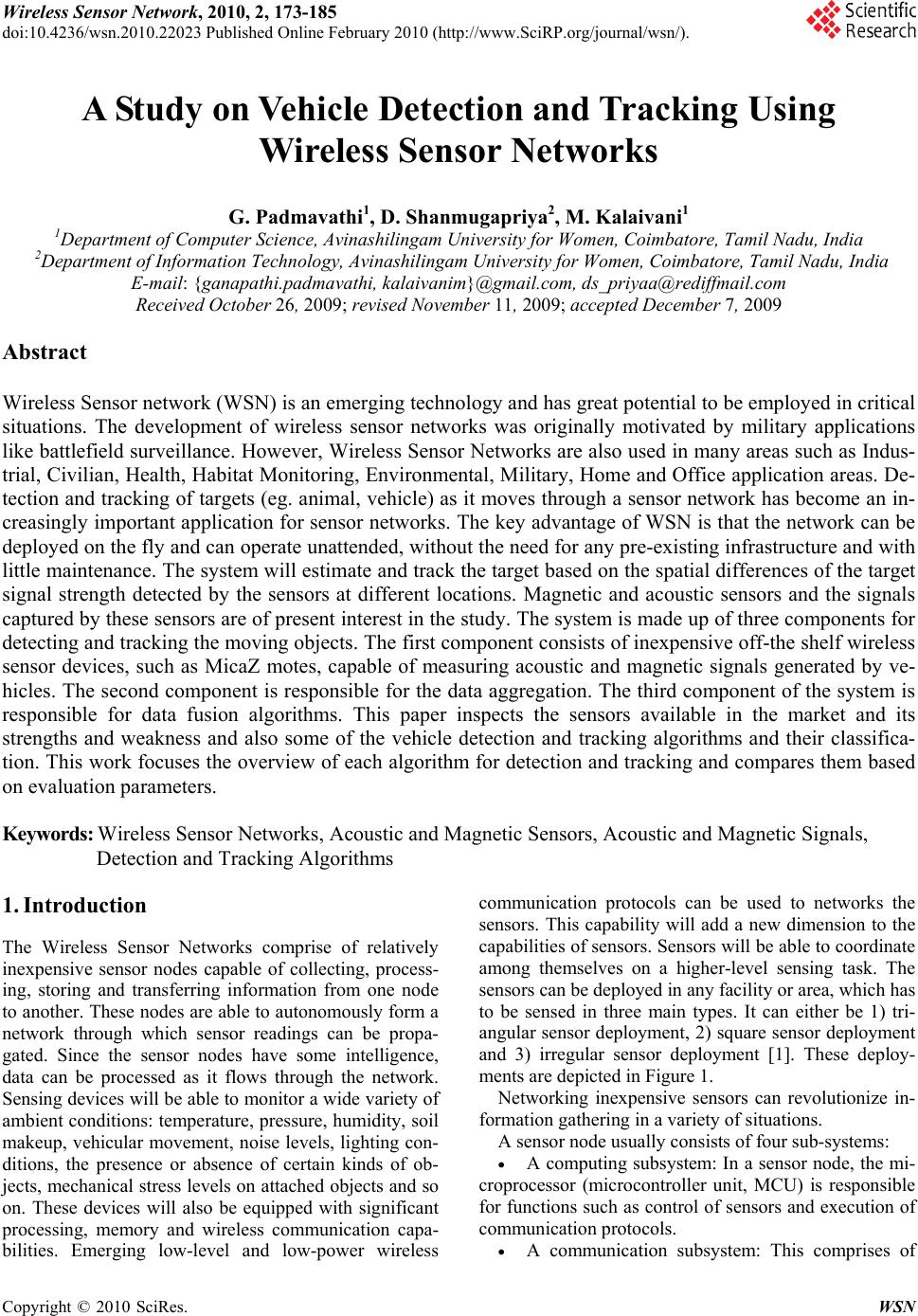Wireless Sensor Network, 2010, 2, 173-185
doi:10.4236/wsn.2010.22023 ublished Online February 2010 (http://www.SciRP.org/journal/wsn/). P
A Study on Vehicle Detection and Tracking Using
Wireless Sensor Networks
G. Padmavathi1, D. Shanmugapriya2, M. Kalaivani1
1Department of Computer Science, Avinashilingam University for Women, Coimbatore, Tamil Nadu, India
2
Department of Information Technology, Avinashilingam University for Women, Coimbatore, Tamil Nadu, India
Received October 26, 2009; revised November 11, 2009; accepted December 7, 2009
Abstract
Wireless Sensor network (WSN) is an emerging technology and has great potential to be employed in critical
situations. The development of wireless sensor networks was originally motivated by military applications
like battlefield surveillance. However, Wireless Sensor Networks are also used in many areas such as Indus-
trial, Civilian, Health, Habitat Monitoring, Environmental, Military, Home and Office application areas. De-
tection and tracking of targets (eg. animal, vehicle) as it moves through a sensor network has become an in-
creasingly important application for sensor networks. The key advantage of WSN is that the network can be
deployed on the fly and can operate unattended, without the need for any pre-existing infrastructure and with
little maintenance. The system will estimate and track the target based on the spatial differences of the target
signal strength detected by the sensors at different locations. Magnetic and acoustic sensors and the signals
captured by these sensors are of present interest in the study. The system is made up of three components for
detecting and tracking the moving objects. The first component consists of inexpensive off-the shelf wireless
sensor devices, such as MicaZ motes, capable of measuring acoustic and magnetic signals generated by ve-
hicles. The second component is responsible for the data aggregation. The third component of the system is
responsible for data fusion algorithms. This paper inspects the sensors available in the market and its
strengths and weakness and also some of the vehicle detection and tracking algorithms and their classifica-
tion. This work focuses the overview of each algorithm for detection and tracking and compares them based
on evaluation parameters.
Keywords: Wireless Sensor Networks, Acoustic and Magnetic Sensors, Acoustic and Magnetic Signals,
Detection and Tracking Algorithms
1. Introduction
The Wireless Sensor Networks comprise of relatively
inexpensive sensor nodes capable of collecting, process-
ing, storing and transferring information from one node
to another. These nodes are able to autonomously form a
network through which sensor readings can be propa-
gated. Since the sensor nodes have some intelligence,
data can be processed as it flows through the network.
Sensing devices will be able to monitor a wide variety of
ambient conditions: temperature, pressure, humidity, soil
makeup, vehicular movement, noise levels, lighting con-
ditions, the presence or absence of certain kinds of ob-
jects, mechanical stress levels on attached objects and so
on. These devices will also be equipped with significant
processing, memory and wireless communication capa-
bilities. Emerging low-level and low-power wireless
communication protocols can be used to networks the
sensors. This capability will add a new dimension to the
capabilities of sensors. Sensors will be able to coordinate
among themselves on a higher-level sensing task. The
sensors can be deployed in any facility or area, which has
to be sensed in three main types. It can either be 1) tri-
angular sensor deployment, 2) square sensor deployment
and 3) irregular sensor deployment [1]. These deploy-
ments are depicted in Figure 1.
Networking inexpensive sensors can revolutionize in-
formation gathering in a variety of situations.
A sensor node usually consists of four sub-systems:
 A computing subsystem: In a sensor node, the mi-
croprocessor (microcontroller unit, MCU) is responsible
for functions such as control of sensors and execution of
communication protocols.
 A communication subsystem: This comprises of

G. PADMAVATHI ET AL. 174
(a) (b) (c)
Figure 1. (a) Triangular; (b) Square; (c) Irregular deployments.
short range radios used to communicate with neighbour-
ing nodes and the outside world. These devices operate
under the Transmit, Receive, Idle and Sleep modes hav-
ing various levels of energy consumption.
 A sensing subsystem: Low power components can
help to significantly reduce power consumption. Since
this subsystem (sensors and actuators) is responsible for
the sharing of information between the sensor network
and the outside world.
 A power supply subsystem: It consists of a battery
which supplies power to the node.
1.1. Characteristics of WSN
Some of the unique characteristics of a WSN include:
 Limited power they can harvest or store.
 Ability to withstand harsh environmental conditions
 Ability to cope with node failures
 Mobility of nodes
 Dynamic network topology
 Communication failures
 Heterogeneity of nodes Large scale of deployment
 Unattended operation
1.2. Applications
The various sensor network applications include,
1) Military Applications
 Monitoring Friendly Forces, Equipments and
Ammunition
 Battlefield Surveillance
 Targeting
 Battle Damage Assessment
 Nuclear, Biological and Chemical Attack Detection
2) Environmental Applications
 Forest Fire Detection
 Flood Detection
 Monitoring through Internet
 Monitoring Biodiversity
3) Habitat Monitoring Applications
 Habitat Monitoring
 Great Duck Island System
4) Health Applications
 Tele-monitoring of Physical Data
 Tracking and Monitoring Doctors and Patients in a
Hospital
 Drug Administration in Hospitals
5) Home and office Applications
 Smart Homes
 Managing Inventory Control
 Home automation
 Environmental control in office buildings
6) Other Applications
 Monitoring Nuclear Reactor.
 Target Tracking
 Suspicious Individual detection: Interactive mu-
seums
 Fire Fighters Problem (First Responders Problem)
The major contribution of this paper includes classifi-
cation of sensors available and vehicle detection and
tracking algorithms using Wireless Sensor Networks.
The paper is organized as follows: Section 2 gives the
classification of sensors used for vehicle detection and
mainly concentrates on the acoustic and magnetic sen-
sors. Section 3 gives the gist about the acoustic and
magnetic signals acquired from the sensors. Section 4
discusses the various algorithms used in vehicle detec-
tion and tracking, analysis about these algorithms is
given in Section 5 and summary of these algorithms
given in Section 6 followed by the conclusion.
2. Classification of Sensors Used in Vehicle
Detection
There are a wide variety of sensors available in market
today [2]. Table 1 shows the variety of current sensor
technologies and compares the strengths and weaknesses
with respect to installation, parameters measured, and per-
formance in bad weather, variable lighting, and changeable
traffic flow. Many over-roadway sensors are compact and
mounted above or the side of the roadway, making installa-
tion and maintenance relatively easy. Some sensor installa-
tion and maintenance applications may require the closing
of the roadway to normal traffic to ensure the safety of the
installer and motorist. All the sensors listed here operate
under day and night conditions. Sensors are broadly classi-
fied as Intrusive and Non-Intrusive sensors.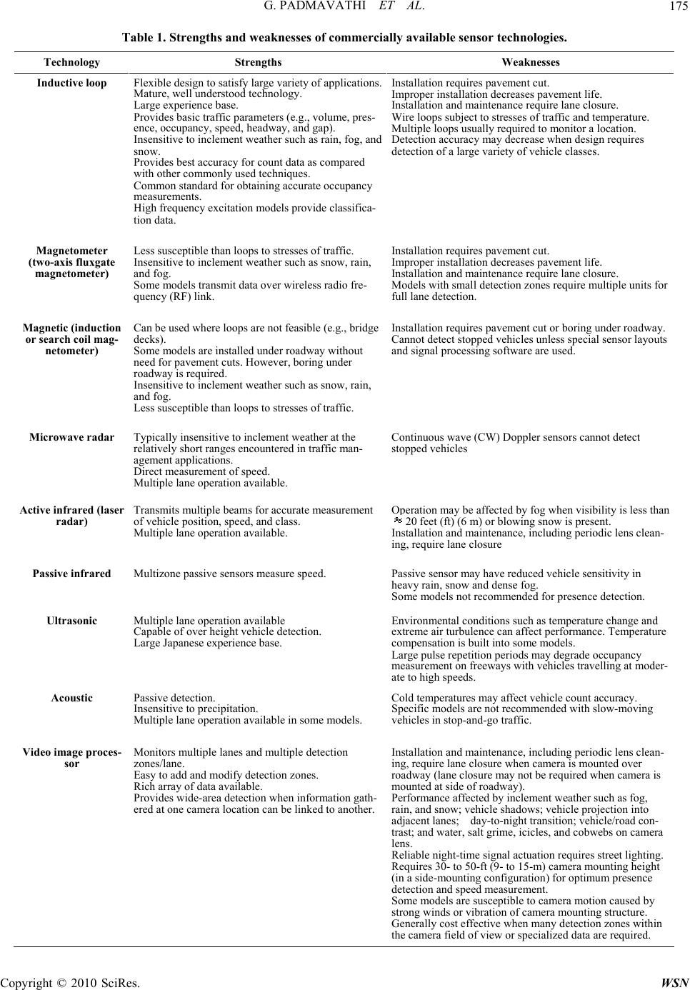

G. PADMAVATHI ET AL.175
Table 1. Strengths and weaknesses of commercially available sensor technologies.
Technology Strengths Weaknesses
Inductive loop Flexible design to satisfy large variety of applications.
Mature, well understood technology.
Large experience base.
Provides basic traffic parameters (e.g., volume, pres-
ence, occupancy, speed, headway, and gap).
Insensitive to inclement weather such as rain, fog, and
snow.
Provides best accuracy for count data as compared
with other commonly used techniques.
Common standard for obtaining accurate occupancy
measurements.
High frequency excitation models provide classifica-
tion data.
Installation requires pavement cut.
Improper installation decreases pavement life.
Installation and maintenance require lane closure.
Wire loops subject to stresses of traffic and temperature.
Multiple loops usually required to monitor a location.
Detection accuracy may decrease when design requires
detection of a large variety of vehicle classes.
Magnetometer
(two-axis fluxgate
magnetometer)
Less susceptible than loops to stresses of traffic.
Insensitive to inclement weather such as snow, rain,
and fog.
Some models transmit data over wireless radio fre-
quency (RF) link.
Installation requires pavement cut.
Improper installation decreases pavement life.
Installation and maintenance require lane closure.
Models with small detection zones require multiple units for
full lane detection.
Magnetic (induction
or search coil mag-
netometer)
Can be used where loops are not feasible (e.g., bridge
decks).
Some models are installed under roadway without
need for pavement cuts. However, boring under
roadway is required.
Insensitive to inclement weather such as snow, rain,
and fog.
Less susceptible than loops to stresses of traffic.
Installation requires pavement cut or boring under roadway.
Cannot detect stopped vehicles unless special sensor layouts
and signal processing software are used.
Microwave radar Typically insensitive to inclement weather at the
relatively short ranges encountered in traffic man-
agement applications.
Direct measurement of speed.
Multiple lane operation available.
Continuous wave (CW) Doppler sensors cannot detect
stopped vehicles
Active infrared (laser
radar)
Transmits multiple beams for accurate measurement
of vehicle position, speed, and class.
Multiple lane operation available.
Operation may be affected by fog when visibility is less than
20 feet (ft) (6 m) or blowing snow is present.
Installation and maintenance, including periodic lens clean-
ing, require lane closure
Passive infrared Multizone passive sensors measure speed. Passive sensor may have reduced vehicle sensitivity in
heavy rain, snow and dense fog.
Some models not recommended for presence detection.
Ultrasonic Multiple lane operation available
Capable of over height vehicle detection.
Large Japanese experience base.
Environmental conditions such as temperature change and
extreme air turbulence can affect performance. Temperature
compensation is built into some models.
Large pulse repetition periods may degrade occupancy
measurement on freeways with vehicles travelling at moder-
ate to high speeds.
Acoustic Passive detection.
Insensitive to precipitation.
Multiple lane operation available in some models.
Cold temperatures may affect vehicle count accuracy.
Specific models are not recommended with slow-moving
vehicles in stop-and-go traffic.
Video image proces-
sor
Monitors multiple lanes and multiple detection
zones/lane.
Easy to add and modify detection zones.
Rich array of data available.
Provides wide-area detection when information gath-
ered at one camera location can be linked to another.
Installation and maintenance, including periodic lens clean-
ing, require lane closure when camera is mounted over
roadway (lane closure may not be required when camera is
mounted at side of roadway).
Performance affected by inclement weather such as fog,
rain, and snow; vehicle shadows; vehicle projection into
adjacent lanes; day-to-night transition; vehicle/road con-
trast; and water, salt grime, icicles, and cobwebs on camera
lens.
Reliable night-time signal actuation requires street lighting.
Requires 30- to 50-ft (9- to 15-m) camera mounting height
(in a side-mounting configuration) for optimum presence
detection and speed measurement.
Some models are susceptible to camera motion caused by
strong winds or vibration of camera mounting structure.
Generally cost effective when many detection zones within
the camera field of view or specialized data are required.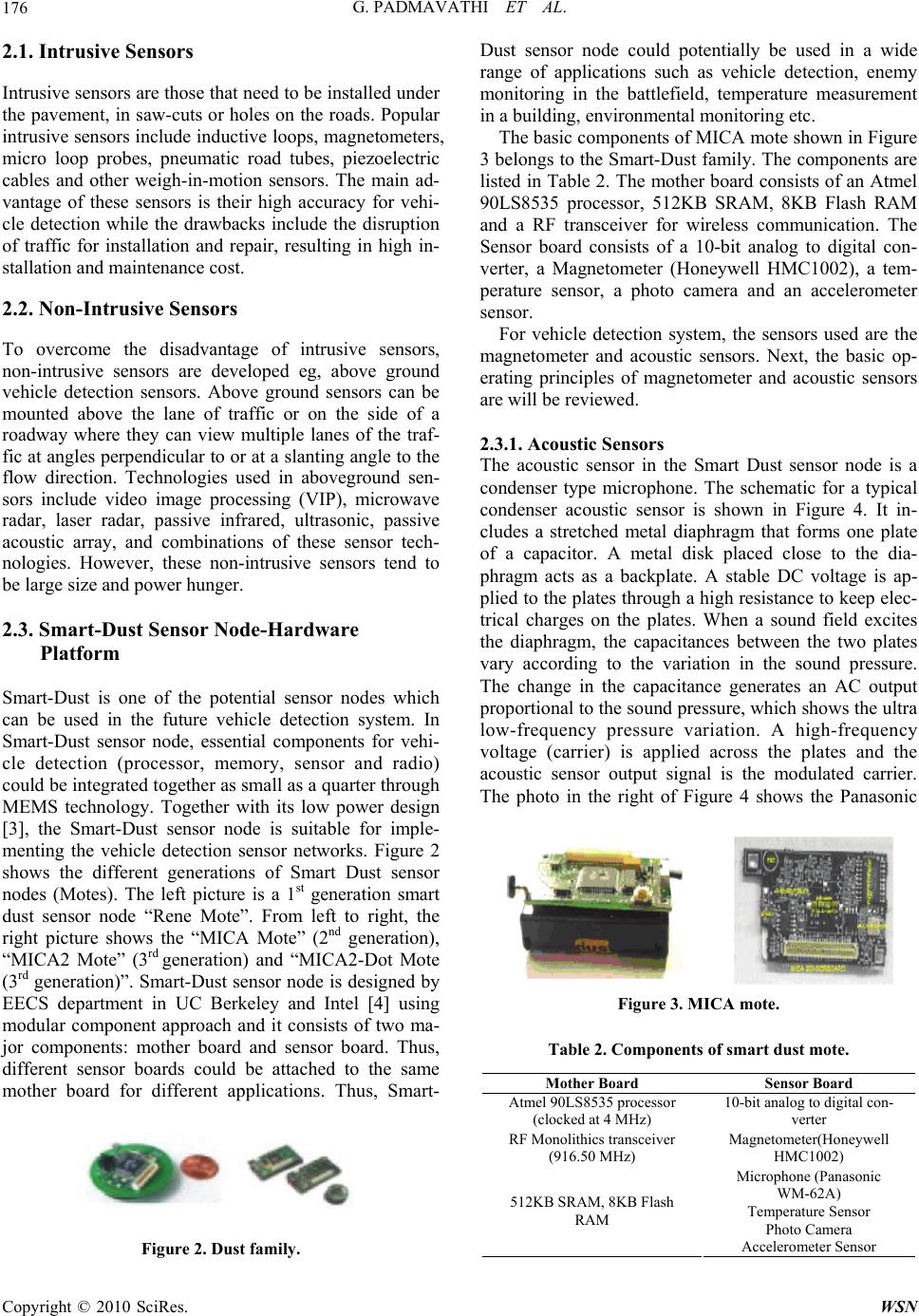

G. PADMAVATHI ET AL. 176
2.1. Intrusive Sensors
Intrusive sensors are those that need to be installed under
the pavement, in saw-cuts or holes on the roads. Popular
intrusive sensors include inductive loops, magnetometers,
micro loop probes, pneumatic road tubes, piezoelectric
cables and other weigh-in-motion sensors. The main ad-
vantage of these sensors is their high accuracy for vehi-
cle detection while the drawbacks include the disruption
of traffic for installation and repair, resulting in high in-
stallation and maintenance cost.
2.2. Non-Intrusive Sensors
To overcome the disadvantage of intrusive sensors,
non-intrusive sensors are developed eg, above ground
vehicle detection sensors. Above ground sensors can be
mounted above the lane of traffic or on the side of a
roadway where they can view multiple lanes of the traf-
fic at angles perpendicular to or at a slanting angle to the
flow direction. Technologies used in aboveground sen-
sors include video image processing (VIP), microwave
radar, laser radar, passive infrared, ultrasonic, passive
acoustic array, and combinations of these sensor tech-
nologies. However, these non-intrusive sensors tend to
be large size and power hunger.
2.3. Smart-Dust Sensor Node-Hardware
Platform
Smart-Dust is one of the potential sensor nodes which
can be used in the future vehicle detection system. In
Smart-Dust sensor node, essential components for vehi-
cle detection (processor, memory, sensor and radio)
could be integrated together as small as a quarter through
MEMS technology. Together with its low power design
[3], the Smart-Dust sensor node is suitable for imple-
menting the vehicle detection sensor networks. Figure 2
shows the different generations of Smart Dust sensor
nodes (Motes). The left picture is a 1st generation smart
dust sensor node “Rene Mote”. From left to right, the
right picture shows the “MICA Mote” (2nd generation),
“MICA2 Mote” (3rd generation) and “MICA2-Dot Mote
(3rd generation)”. Smart-Dust sensor node is designed by
EECS department in UC Berkeley and Intel [4] using
modular component approach and it consists of two ma-
jor components: mother board and sensor board. Thus,
different sensor boards could be attached to the same
mother board for different applications. Thus, Smart-
Figure 2. Dust family.
Dust sensor node could potentially be used in a wide
range of applications such as vehicle detection, enemy
monitoring in the battlefield, temperature measurement
in a building, environmental monitoring etc.
The basic components of MICA mote shown in Figure
3 belongs to the Smart-Dust family. The components are
listed in Table 2. The mother board consists of an Atmel
90LS8535 processor, 512KB SRAM, 8KB Flash RAM
and a RF transceiver for wireless communication. The
Sensor board consists of a 10-bit analog to digital con-
verter, a Magnetometer (Honeywell HMC1002), a tem-
perature sensor, a photo camera and an accelerometer
sensor.
For vehicle detection system, the sensors used are the
magnetometer and acoustic sensors. Next, the basic op-
erating principles of magnetometer and acoustic sensors
are will be reviewed.
2.3.1. Acoustic Sensors
The acoustic sensor in the Smart Dust sensor node is a
condenser type microphone. The schematic for a typical
condenser acoustic sensor is shown in Figure 4. It in-
cludes a stretched metal diaphragm that forms one plate
of a capacitor. A metal disk placed close to the dia-
phragm acts as a backplate. A stable DC voltage is ap-
plied to the plates through a high resistance to keep elec-
trical charges on the plates. When a sound field excites
the diaphragm, the capacitances between the two plates
vary according to the variation in the sound pressure.
The change in the capacitance generates an AC output
proportional to the sound pressure, which shows the ultra
low-frequency pressure variation. A high-frequency
voltage (carrier) is applied across the plates and the
acoustic sensor output signal is the modulated carrier.
The photo in the right of Figure 4 shows the Panasonic
Figure 3. MICA mote.
Table 2. Components of smart dust mote.
Mother Board Sensor Board
Atmel 90LS8535 processor
(clocked at 4 MHz)
10-bit analog to digital con-
verter
RF Monolithics transceiver
(916.50 MHz)
Magnetometer(Honeywell
HMC1002)
Microphone (Panasonic
WM-62A)
Temperature Sensor
Photo Camera
512KB SRAM, 8KB Flash
RAM
Accelerometer Sensor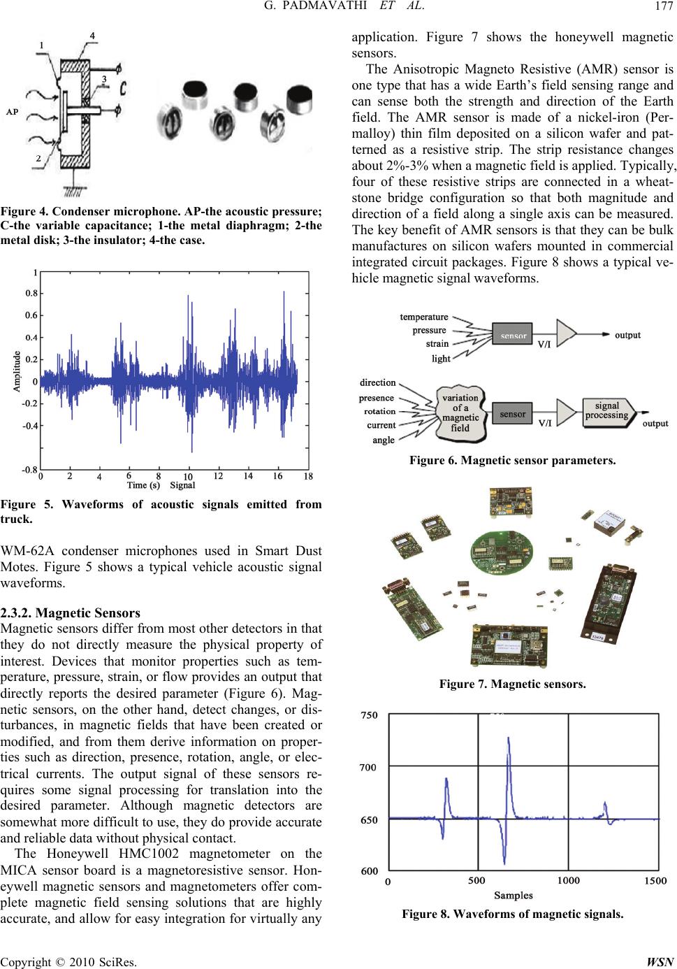

G. PADMAVATHI ET AL.177
Figure 4. Condenser microphone. AP-the acoustic pressure;
C-the variable capacitance; 1-the metal diaphragm; 2-the
metal disk; 3-the insulator; 4-the case.
Figure 5. Waveforms of acoustic signals emitted from
truck.
WM-62A condenser microphones used in Smart Dust
Motes. Figure 5 shows a typical vehicle acoustic signal
waveforms.
2.3.2. Magnetic Sensors
Magnetic sensors differ from most other detectors in that
they do not directly measure the physical property of
interest. Devices that monitor properties such as tem-
perature, pressure, strain, or flow provides an output that
directly reports the desired parameter (Figure 6). Mag-
netic sensors, on the other hand, detect changes, or dis-
turbances, in magnetic fields that have been created or
modified, and from them derive information on proper-
ties such as direction, presence, rotation, angle, or elec-
trical currents. The output signal of these sensors re-
quires some signal processing for translation into the
desired parameter. Although magnetic detectors are
somewhat more difficult to use, they do provide accurate
and reliable data without physical contact.
The Honeywell HMC1002 magnetometer on the
MICA sensor board is a magnetoresistive sensor. Hon-
eywell magnetic sensors and magnetometers offer com-
plete magnetic field sensing solutions that are highly
accurate, and allow for easy integration for virtually any
application. Figure 7 shows the honeywell magnetic
sensors.
The Anisotropic Magneto Resistive (AMR) sensor is
one type that has a wide Earth’s field sensing range and
can sense both the strength and direction of the Earth
field. The AMR sensor is made of a nickel-iron (Per-
malloy) thin film deposited on a silicon wafer and pat-
terned as a resistive strip. The strip resistance changes
about 2%-3% when a magnetic field is applied. Typically,
four of these resistive strips are connected in a wheat-
stone bridge configuration so that both magnitude and
direction of a field along a single axis can be measured.
The key benefit of AMR sensors is that they can be bulk
manufactures on silicon wafers mounted in commercial
integrated circuit packages. Figure 8 shows a typical ve-
hicle magnetic signal waveforms.
Figure 6. Magnetic sensor parameters.
Figure 7. Magnetic sensors.
Figure 8. Waveforms of magnetic signals.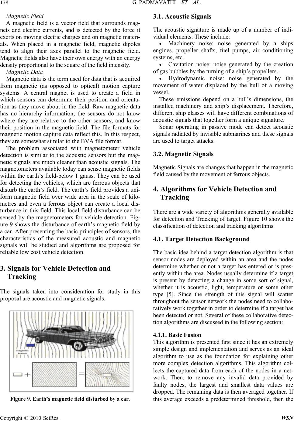

G. PADMAVATHI ET AL. 178
Magnetic Field
A magnetic field is a vector field that surrounds mag-
nets and electric currents, and is detected by the force it
exerts on moving electric charges and on magnetic materi-
als. When placed in a magnetic field, magnetic dipoles
tend to align their axes parallel to the magnetic field.
Magnetic fields also have their own energy with an energy
density proportional to the square of the field intensity.
Magnetic Data
Magnetic data is the term used for data that is acquired
from magnetic (as opposed to optical) motion capture
systems. A central magnet is used to create a field in
which sensors can determine their position and orienta-
tion as they move about in the field. Raw magnetic data
has no hierarchy information; the sensors do not know
where they are relative to the other sensors, and know
their position in the magnetic field. The file formats for
magnetic motion capture data reflect this. In this respect,
they are somewhat similar to the BVA file format.
The problem associated with magnetometer vehicle
detection is similar to the acoustic sensors but the mag-
netic signals are much cleaner than acoustic signals. The
magnetometers available today can sense magnetic fields
within the earth’s field-below 1 gauss. They can be used
for detecting the vehicles, which are ferrous objects that
disturb the earth’s field. The earth’s field provides a uni-
form magnetic field over wide area in the scale of kilo-
metres and even a ferrous object can create a local dis-
turbance in this field. This local field disturbance can be
sensed by the magnetometers for vehicle detection. Fig-
ure 9 shows the disturbance of earth’s magnetic field by
a car. After presenting the basic principles of sensors, the
characteristics of the measured acoustic and magnetic
signals will be studied and algorithms are proposed for
reliable low cost vehicle detection.
3. Signals for Vehicle Detection and
Tracking
The signals taken into consideration for study in this
proposal are acoustic and magnetic signals.
Figure 9. Earth’s magnetic field disturbed by a car.
3.1. Acoustic Signals
The acoustic signature is made up of a number of indi-
vidual elements. These include:
 Machinery noise: noise generated by a ships
engines, propeller shafts, fuel pumps, air conditioning
systems, etc.
 Cavitation noise: noise generated by the creation
of gas bubbles by the turning of a ship’s propellers.
 Hydrodynamic noise: noise generated by the
movement of water displaced by the hull of a moving
vessel.
These emissions depend on a hull’s dimensions, the
installed machinery and ship’s displacement. Therefore,
different ship classes will have different combinations of
acoustic signals that together form a unique signature.
Sonar operating in passive mode can detect acoustic
signals radiated by invisible submarines and these signals
are used to target attacks.
3.2. Magnetic Signals
Magnetic Signals are changes that happen in the magnetic
field caused by the movement of ferrous objects.
4. Algorithms for Vehicle Detection and
Tracking
There are a wide variety of algorithms generally available
for detection and Tracking of target. Figure 10 shows the
classification of detection and tracking algorithms.
4.1. Target Detection Background
The basic idea behind a target detection algorithm is that
sensor nodes are deployed within an area and the nodes
determine whether or not a target has entered or is pres-
ently within the area. Nodes usually determine if a target
is present by detecting a change in some sort of signal,
whether it is acoustic, light, temperature or some other
type [5]. Since the strength of this signal will scatter
throughout the sensor network the nodes need to collabo-
ratively work together in order to determine if a target has
been detected or not. Several of these collaborative detec-
tion algorithms are discussed in the following section:
4.1.1. Basic Fusion
This algorithm is presented first since it has an extremely
simple design and implementation and serves as an ideal
algorithm to use as the foundation for explaining other
more complex detection algorithms. This algorithm col-
lects the captured data from each of the nodes in a net-
work. Then, to remove any invalid data provided by
faulty nodes, the largest and smallest data values are
dropped. The remaining data is then averaged together. If
this average exceeds a predetermined threshold, then the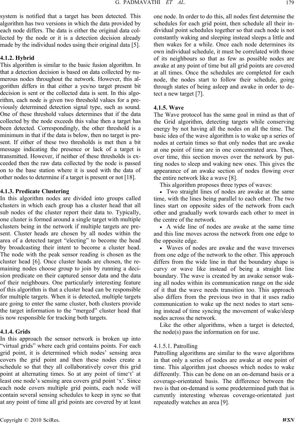

G. PADMAVATHI ET AL.179
system is notified that a target has been detected. This
algorithm has two versions in which the data provided by
each node differs. The data is either the original data col-
lected by the node or it is a detection decision already
made by the individual nodes using their original data [5].
4.1.2. Hybrid
This algorithm is similar to the basic fusion algorithm. In
that a detection decision is based on data collected by nu-
merous nodes throughout the network. However, this al-
gorithm differs in that either a yes/no target present bit
decision is sent or the collected data is sent. In this algo-
rithm, each node is given two threshold values for a pre-
viously determined detection signal type, such as sound.
One of these threshold values determines that if the data
collected by the node exceeds this value then a target has
been detected. Correspondingly, the other threshold is a
minimum in that if the data is below, then no target is pre-
sent. If either of these two thresholds is met then a bit
message indicating the presence or lack of a target is
transmitted. However, if neither of these thresholds is ex-
ceeded then the raw data collected by the node is passed
on to the base station where it is used with the data of
other nodes to determine if a target is present or not [18].
4.1.3. Predicate Clustering
In this algorithm nodes are divided into groups called
clusters in which each group has a cluster head that all
sub nodes of the cluster report their data to. Typically,
one cluster is formed around a single target with multiple
clusters being in the network if multiple targets are pre-
sent. Cluster heads are chosen by all nodes within the
area of a detected target “electing” to become the head
by broadcasting their intent to become a cluster head.
The node with the peak sensor reading is chosen as the
cluster head [6]. Once cluster heads are chosen, the re-
maining nodes choose group to join by running a deci-
sion predicate on their captured sensor data and the data
of their neighbours. One particularly interesting feature
of this algorithm is that a cluster head can be responsible
for multiple targets. When it is detected, multiple targets
are going to enter the same cluster, both clusters provide
the target information to the “merged” cluster head that
is now responsible for tracking both targets.
4.1.4. Grids
In this approach the sensor network is broken up into
“virtual grids” where each grid contains points. For each
grid point, it is determined which nodes’ sensing area
covers the grid point and then these nodes create a
schedule so that they all collaboratively cover this grid
point at alternating times. So at any point of time‘t’ at
least one node’s sensing area covers grid point ‘x’. Since
each node covers multiple grid points, each node will
contain several sensing schedules to keep in sync so that
at any point of time all grid points are covered by at least
one node. In order to do this, all nodes first determine the
schedules for each grid point, then schedule all their in-
dividual point schedules together so that each node is not
constantly waking and sleeping instead sleeps a little and
then wakes for a while. Once each node determines its
own individual schedule, it must be correlated with those
of its neighbours so that as few as possible nodes are
awake at any point of time but all grid points are covered
at all times. Once the schedules are completed for each
node, the nodes start to follow their schedule, going
through states of being asleep and awake in order to de-
tect a new target [7].
4.1.5. Wave
The Wave protocol has the same goal in mind as that of
the Grid algorithm, detecting targets while conserving
energy by not having all the nodes on all the time. The
basic idea of the wave algorithm is to wake up a series of
nodes at certain times so that only nodes that are awake
at one point of time are in one concentrated area. Then,
over time, this section moves over the network by put-
ting nodes to sleep and waking new ones. This gives the
appearance of an awake section of nodes flowing over
the entire network like a wave [8].
This algorithm proposes three types of waves:
 Two straight lines of nodes are awake at the same
time, with the lines being parallel to each other. The two
lines start on opposite sides of the network from each
other and gradually work towards each other to meet in
the centre of the network.
 A wide line of nodes are awake at the same time
and this line moves across the network from one edge to
the opposite edge.
 Waves of nodes are awake and the wave traverses
from one edge of the network to the other. This approach
differs from the wide line in that the boundary shape is
curvy or wave like instead of being a straight line
boundary. The wave is created by an awake sensor wak-
ing all nodes within its communication range on the side
of it that the wave needs transition too. This approach
also differs from the previous two in that it uses radio
communication to wake up the next nodes to start sens-
ing instead of time syncing the movement of wake/sleep
nodes across the network.
Like the other algorithms, when a target is detected,
the node(s) pass the information on for use.
4.1.5.1. Patrolling
Patrolling algorithms are similar to the wave algorithms
in that only a series of nodes are awake at one point of
time. This algorithm just chooses which nodes to wake
differently. This can be done on an on-demand basis or a
coverage-orientated basis. The difference between the
two is that on-demand is some predetermined path that is
currently interesting whereas coverage-orientated just
repeatedly watches an area [9].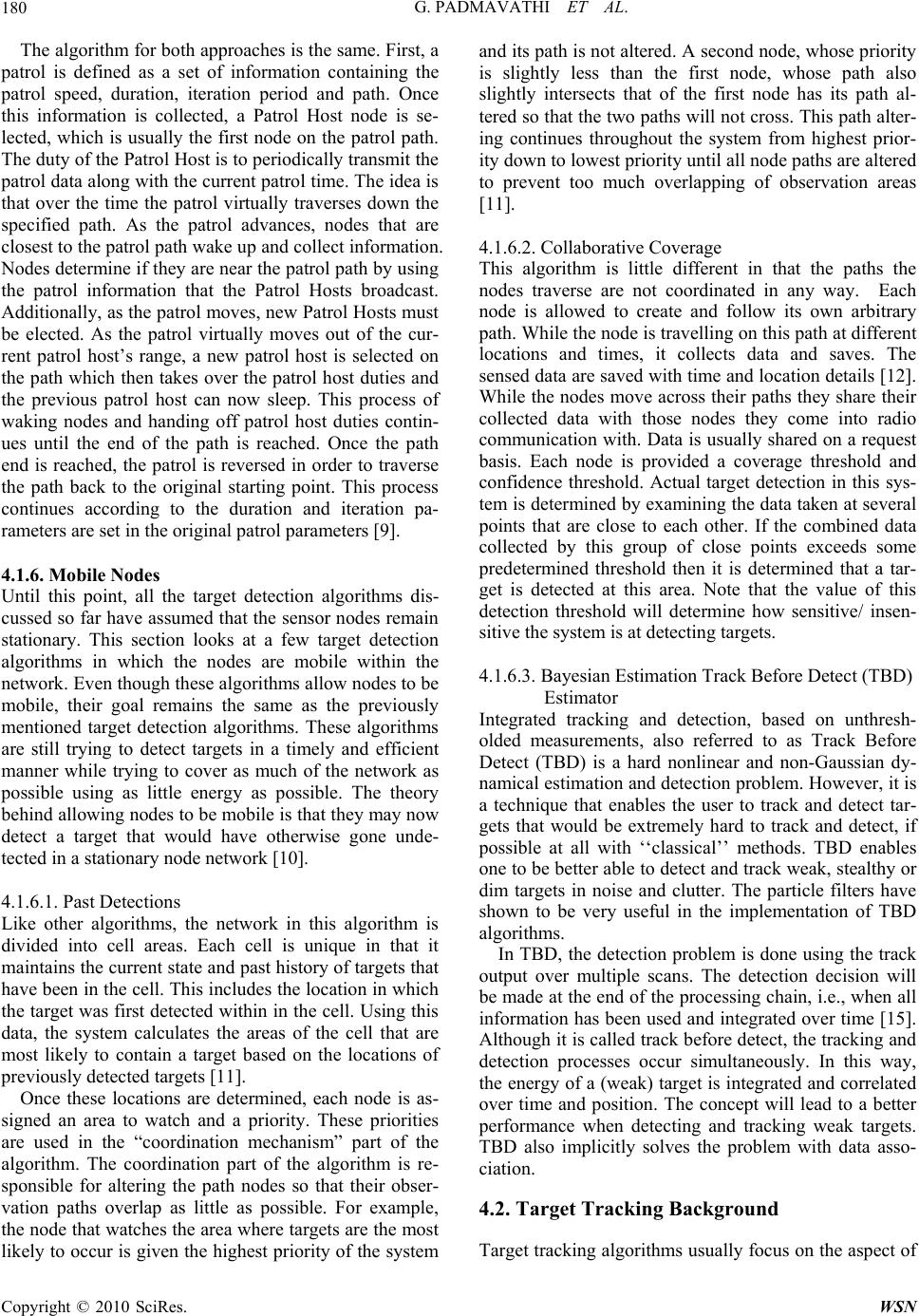

G. PADMAVATHI ET AL. 180
The algorithm for both approaches is the same. First, a
patrol is defined as a set of information containing the
patrol speed, duration, iteration period and path. Once
this information is collected, a Patrol Host node is se-
lected, which is usually the first node on the patrol path.
The duty of the Patrol Host is to periodically transmit the
patrol data along with the current patrol time. The idea is
that over the time the patrol virtually traverses down the
specified path. As the patrol advances, nodes that are
closest to the patrol path wake up and collect information.
Nodes determine if they are near the patrol path by using
the patrol information that the Patrol Hosts broadcast.
Additionally, as the patrol moves, new Patrol Hosts must
be elected. As the patrol virtually moves out of the cur-
rent patrol host’s range, a new patrol host is selected on
the path which then takes over the patrol host duties and
the previous patrol host can now sleep. This process of
waking nodes and handing off patrol host duties contin-
ues until the end of the path is reached. Once the path
end is reached, the patrol is reversed in order to traverse
the path back to the original starting point. This process
continues according to the duration and iteration pa-
rameters are set in the original patrol parameters [9].
4.1.6. Mobile Nodes
Until this point, all the target detection algorithms dis-
cussed so far have assumed that the sensor nodes remain
stationary. This section looks at a few target detection
algorithms in which the nodes are mobile within the
network. Even though these algorithms allow nodes to be
mobile, their goal remains the same as the previously
mentioned target detection algorithms. These algorithms
are still trying to detect targets in a timely and efficient
manner while trying to cover as much of the network as
possible using as little energy as possible. The theory
behind allowing nodes to be mobile is that they may now
detect a target that would have otherwise gone unde-
tected in a stationary node network [10].
4.1.6.1. Past Detections
Like other algorithms, the network in this algorithm is
divided into cell areas. Each cell is unique in that it
maintains the current state and past history of targets that
have been in the cell. This includes the location in which
the target was first detected within in the cell. Using this
data, the system calculates the areas of the cell that are
most likely to contain a target based on the locations of
previously detected targets [11].
Once these locations are determined, each node is as-
signed an area to watch and a priority. These priorities
are used in the “coordination mechanism” part of the
algorithm. The coordination part of the algorithm is re-
sponsible for altering the path nodes so that their obser-
vation paths overlap as little as possible. For example,
the node that watches the area where targets are the most
likely to occur is given the highest priority of the system
and its path is not altered. A second node, whose priority
is slightly less than the first node, whose path also
slightly intersects that of the first node has its path al-
tered so that the two paths will not cross. This path alter-
ing continues throughout the system from highest prior-
ity down to lowest priority until all node paths are altered
to prevent too much overlapping of observation areas
[11].
4.1.6.2. Collaborative Coverage
This algorithm is little different in that the paths the
nodes traverse are not coordinated in any way. Each
node is allowed to create and follow its own arbitrary
path. While the node is travelling on this path at different
locations and times, it collects data and saves. The
sensed data are saved with time and location details [12].
While the nodes move across their paths they share their
collected data with those nodes they come into radio
communication with. Data is usually shared on a request
basis. Each node is provided a coverage threshold and
confidence threshold. Actual target detection in this sys-
tem is determined by examining the data taken at several
points that are close to each other. If the combined data
collected by this group of close points exceeds some
predetermined threshold then it is determined that a tar-
get is detected at this area. Note that the value of this
detection threshold will determine how sensitive/ insen-
sitive the system is at detecting targets.
4.1.6.3. Bayesian Estimation Track Before Detect (TBD)
Estimator
Integrated tracking and detection, based on unthresh-
olded measurements, also referred to as Track Before
Detect (TBD) is a hard nonlinear and non-Gaussian dy-
namical estimation and detection problem. However, it is
a technique that enables the user to track and detect tar-
gets that would be extremely hard to track and detect, if
possible at all with ‘‘classical’’ methods. TBD enables
one to be better able to detect and track weak, stealthy or
dim targets in noise and clutter. The particle filters have
shown to be very useful in the implementation of TBD
algorithms.
In TBD, the detection problem is done using the track
output over multiple scans. The detection decision will
be made at the end of the processing chain, i.e., when all
information has been used and integrated over time [15].
Although it is called track before detect, the tracking and
detection processes occur simultaneously. In this way,
the energy of a (weak) target is integrated and correlated
over time and position. The concept will lead to a better
performance when detecting and tracking weak targets.
TBD also implicitly solves the problem with data asso-
ciation.
4.2. Target Tracking Background
Target tracking algorithms usually focus on the aspect of

G. PADMAVATHI ET AL.181
the sensor nodes’ interaction with a target after the target
has already been detected within the area the sensor
nodes cover. Once the object has been detected, the
nodes collect information and then use one of many dif-
ferent types of algorithms to calculate the current loca-
tion of the object relative to the sensor nodes’ locations.
From here, it is the goal of the sensor network to track
the object as it moves through the network. This may or
may not involve predicting the next location of the object
when it moves. In order to forewarn those nodes it will
be heading towards to prepare to capture data [14]. Sev-
eral of these tracking algorithms are discussed in the fol-
lowing section:
4.2.1. Simple Triangulation
This algorithm is an extremely simple design and im-
plementation and serves as an ideal algorithm to use as
the foundation for explaining other more complex track-
ing algorithms. The whole goal of this algorithm [14] is
to provide a simple algorithm that uses simple computa-
tion in order to calculate an object’s current location and
predict where it is headed and notify those nodes near the
predicted next location of the object.
This algorithm first assumes that all nodes in the
network are localized to a common reference point and
can detect and estimate the distance to a target using
signal strength [14]. When a node detects an object
within its range it broadcasts a TargetDetected message.
This message contains the location of the sensor node
and the distance to the target. All nodes that hear this
message store its data in their local memory. When a
node that has detected the target hears two other Tar-
getDetected messages from two other nodes it performs
triangulation on the three coordinates to calculate the
location of the target. (Note that this means that more
than one node may perform this calculation for the
same target at the same time.) This node then continues
to project the trajectory of the target. When the esti-
mated target trajectory has been calculated, all nodes
that are within some distance ‘d’ perpendicular to the
target’s trajectory are sent a Warning message to alert
them that the target is headed towards them. These
newly awoken nodes then track the object as it enters
their area and repeat the TargetDetected and Warning
message sending process.
4.2.2. Clusters
The cluster target tracking algorithm has been widely
discussed through many research papers. In this section,
the basic idea of target tracking using clusters is dis-
cussed, followed by an overview of the variances in each
of the different cluster algorithm research papers.
4.2.2.1. Basic Cluster Algorithm
The basic algorithm for tracking an object using clusters
is as follows [20]:
 Some (or all) of the nodes in a cluster detect the
object and report their data to a cluster head. Note that
each cluster has only one cluster head.
 The cluster head node uses all the target detection
information from the sensor nodes to estimate the tar-
get’s location.
 The cluster head uses the calculated target location
and past locations of the target to predict the next loca-
tion of the target.
 Those sensors around the predicted location are
woken up to form a new cluster (if not already in one) to
detect the target.
 When the target is detected in this new cluster, the
previous cluster’s nodes are all put into a sleep state.
This new cluster then continues the cluster tracking algo-
rithm.
4.2.2.2. Hierarchical Supernodes
This algorithm deviates from the basic algorithm in that
the cluster heads (called supernodes) have a higher
communication range and more computational power
[21]. These “supernodes” are distributed throughout the
network and the otherwise normal nodes are assigned to
supernodes. Clusters are not dynamically generated in
this algorithm. Interestingly enough, supernodes do share
target location information among each other, whereas
regular sensor nodes do not.
4.2.2.3. Dynamic Clustering
Like the supernode algorithm, this algorithm also as-
sumes that cluster head nodes have more power than
normal sensor nodes. However, sensor nodes are not
assigned to clusters in this algorithm. Instead, they are
invited to join a cluster by the cluster head. The cluster
head does this by broadcasting a join message that in-
cludes the time and signature of the target the cluster
head detected [19]. Those sensor nodes that have stored
data that matches the data in the broadcast message re-
spond to the broadcast by sending their captured data to
the cluster head node. Interestingly, the cluster head only
waits for a certain number of replies and when the re-
quired numbers of replies are received, the cluster head
calculates the target’s location. Unlike the supernode
algorithm, this algorithm has one active cluster head at a
time. In other words, cluster heads do not work together
[22].
4.2.2.4. Cell Collaboration
Like predicate clustering all nodes in this algorithm are
of the same type. Nodes are formed into clusters (called
cells) in which all nodes within the cells collaboratively
decide when a target has entered their cell and if they
should track it [22]. It is interesting to note that cells can
have different sizes; the size of cells is determined by the
observed velocity of the target. So cell size will increase
for faster moving targets.

G. PADMAVATHI ET AL. 182
4.2.2.5. Probabilistic Localization
This algorithm deviates even further from the previously
discussed algorithms. Cluster heads are special high
powered nodes that know the location of every node
within their cluster [23]. This algorithm takes advantage
of the fact that the cluster head knows these locations.
When sensor nodes detect a target, they send a very
small notification message to their cluster head and store
the target location data, time and other relevant data in
their local memory. Upon receiving several notifications,
the cluster head performs a probabilistic localization al-
gorithm to determine which sensor nodes to query saved
data from. In other words, the cluster head runs an algo-
rithm that helps to predict which sensor nodes are closest
to the target. Therefore, the cluster head has the best data
to calculate an accurate estimation of the target location.
When the cluster head determines which nodes to query,
they are asked for the data they saved in their local
memory and the cluster head uses this information to
calculate the location of the target.
4.2.2.6. Distributes Predictive Tracking
This algorithm is very similar to the predicate localiza-
tion algorithm in that cluster head knows the ID, location
and energy level of each of the nodes within their cluster.
However, not all nodes belong to a cluster. Nodes on the
border of the network are not in a cluster and those are
on sense at all times. Similarly, nodes next to the border
are not in a cluster. Moreover the, cluster heads only
choose 3 nodes from target tracking data. Cluster heads
determine which 3 nodes to query based on their location
in relation to the predicted target location calculated by a
previous cluster [24]. When the cluster head has chosen
which nodes to query, those nodes are woken up to pre-
pare to detect the approachable target. This algorithm
differs even further in that if a cluster head cannot find 3
suitable nodes within its own cluster, it can seek the help
of neighbouring clusters and ask for one or more of their
nodes to be turned on and report information.
4.2.3. Rooted Tree
Related to the clusters tracking algorithm is the idea of
the rooted tree tracking algorithm. This algorithm differs
somewhat in that instead of having multiple cluster heads,
there is only one head node and it is referred to as the
root. The root node is the node that is closest to the target.
When a new target location is predicted, if there is an-
other node that is closer to that position than the current
root then new node becomes the root. Other nodes
around the root work together to form a tree in which
their sensed data is collected and passed up through the
tree (children to parents) until all data reaches the root
[25]. When the root receives all the data it calculates the
target position and predicts the new target position as
mentioned in the basic target tracking algorithm. The tree
itself is reconfigured on every root change. When a root
change occurs, a “reconfigure” message is broadcast
containing the location of the new root. When a node
detects the “reconfigure” message, it detaches itself from
the old tree and attaches itself to the new tree by recog-
nizing its neighbour node that is closest to the new root
node as its new parent. New data is then collected and
passed up the tree for the new root to use.
4.2.4. Particle Filtering
The basic idea behind a particle filtering tracking algo-
rithm is that numerous object state descriptions are saved
that contain data necessary to calculate the target posi-
tion at a certain time. These state descriptions are re-
ferred to as particles and each particle has its own weight.
The weight of a particle determines how much the data it
contains will contribute to the location estimation of an
object. When new particles are created, the weights of
the pre-existing particles are adjusted and then all the
particles are used to calculate a new target location [26].
Eventually, particles with weights that are below a cer-
tain threshold are eliminated as duplicate particles.
Some of the particles filtering algorithms differ a little.
Certain algorithms have all the particles stored in a cen-
tral node and this node does all the target location proc-
essing [28]. Other algorithms distribute the stored parti-
cles across the network nodes.
5. Analysis of Algorithms
This section analyses each target tracking algorithm
mentioned with a focus on how it could be improved by
combining it with one or more of the ideas presented in
the target detection algorithms.
5.1. Simple Triangulation
The main problem with this algorithm lies in the fact that
when a node has detected a target and hears two other
nodes broadcast the same target detection, the nodes
starts to perform the triangulation localization calculation.
This means that at the same point of time there will be
multiple nodes calculating the same target location. This
is a waste of computation and energy resources. This
algorithm needs to be improved so that when a node
starts to calculate the location of the target, it first
broadcasts its intention to calculate the location to all the
other nodes, similar to the data sharing that is done in the
collaborative coverage mobile detection algorithm. Then
all the other nodes that would have performed this same
calculation will not perform it once they hear the broad-
casted intention of the first node.
5.2. Basic Cluster
The majority of the cluster algorithms had all the nodes
on during their target detection phase. It would be better
if they instead adopt a technique similar to that used in
the wave detection algorithm to detect targets. Since each

G. PADMAVATHI ET AL.183
area of the network is already divided into clusters, each
node within the cluster could take turns monitoring the
area for the arrival of a target using one of the wave de-
tection methods mentioned. This would increase the life-
time of the network.
However, using one of the mobile detection algorithms
is not recommended since the nodes have to register with
the cluster head. Depending on the mobile detection algo-
rithm used, the nodes would constantly be moving in and
out of clusters. This would cause an increase in the
amount of message communications with these nodes in
order keep track of the nodes within the cluster. Mobile
detection algorithm of this type can be applied to the
situation only if the mobility of the nodes is limited and
the node always stay within the same cluster.
Additionally, the cluster algorithms could benefit from
the basic fusion detection algorithm. Once a target has
been detected and all the information is passed to the
cluster head the cluster head could use the technique
used in the basic fusion algorithm to eliminate any data
provide by faulty nodes. This would help make the net-
work less vulnerable to faulty nodes.
5.2.1. Dynamic Clustering
The biggest problem with this algorithm is that it will not
work with mobile nodes. The network calculates the
sensor node’s locations at start-up. Since these locations
need to be known by the cluster head and are calculated
only once, this prevents any nodes from moving or even
being added to the network. This problem could be easily
fixed by periodically refreshing the locations of the sen-
sor nodes, although this will decrease the network’s life-
time. So it is better to use a detection algorithm and con-
stantly refreshing the nodes’ location isn’t an optimal
solution is better in this case.
5.2.2. Cell Collaboration
This clustering algorithm is already perfectly setup to use
the grid detection algorithm for detection of targets.
Since the nodes in this algorithm are already divided into
cells, the basic structure to use the grid algorithm is al-
ready in place. All that needs to be done is to add the
grid algorithm for the detection part. Once, this is done
the algorithm would be more efficient since the nodes
would be alternating sleep schedules with each other in
order to detect the target instead of all being awake at the
same time.
5.2.3. Probabilistic Localization
This algorithm already sounds like that it has incorpo-
rated parts of the hybrid detection algorithm in it. When
a target is detected, this algorithm sends a small mes-
sage to the cluster head. Similarly, when a target is de-
tected in the hybrid algorithm a small yes/no bit mes-
sage is sent to the decision maker in the network, or
cluster head. Then the cluster head uses this data to
determine which nodes to query for further data. In de-
termining which nodes to query, it would be a good
idea to use an averaging technique similar to that used
in the basic fusion detection algorithm in order to
eliminate the impact of any data provided by a faulty
node. The similarities to the hybrid algorithm continue.
When the cluster head determines which nodes to query,
the nodes respond back to the cluster head with more
detailed information.
However, this algorithm should not be combined with
a mobile node detection algorithm because of the way it
decides which nodes to query. In this algorithm, the
cluster heads create probability tables in order to deter-
mine which sensors to query [23]. The use of a table is
acceptable until nodes move outside or are added to the
system. When this happens, the probability table must be
updated. Therefore, the use of a mobile detection scheme
would cause a lot of additional computational overhead
since these tables are to be constantly refreshed.
5.2.4. Distributed Predictive Tracking
This algorithm is unique in that it is already doing its
own target detecting. Instead of having the border nodes
being on at all times to detect nodes it would be benefi-
cial to have these nodes adopt a wave or patrol like tech-
nique. This way, they would still detect targets but would
be consuming a considerably smaller amount of energy.
5.3. Rooted Tree
One of the basic problems with the rooted tree technique
is that it doesn’t provide any fault tolerance facts. In or-
der to make this algorithm less vulnerable to problems
caused by faulty nodes, it should use an averaging tech-
nique similar to that used in the basic fusion detection
algorithm.
Additionally, this algorithm encounters problems
when the velocity of the target is very high. As the ve-
locity of the target increases so does the number of times
in which the tree must be reconfigured [25]. This will
cause problems when a threshold velocity of the target is
reached in which the tree can no longer be generated
quickly enough to keep up with the moving target. This
problem could be eliminated by altering this algorithm to
work more like the patrolling algorithm. Instead of con-
stantly rebuilding the tree, the tree is treated as a path
that can have steps (or nodes) along the path added or
deleted from it. This way when the target moves, just add
a new node to the path and remove any one that is too far
away to contribute any longer. The basic nodes needed to
collect data are still members of the path and new ones
are added. It saves an enormous amount of time and
message communication needed to periodically rebuild
the tree structure each time.

G. PADMAVATHI ET AL. 184
5.4. Particle Filtering
In order to track targets, this algorithm saves an enor-
mous amount of data in the form of particles. Over time,
these particles take up a large amount of memory space.
The amount of memory actually used could be decreased
if this algorithm is to adopt the idea behind the TBD al-
gorithm. Bayesian Estimation Track Before Detect (TBD)
based on particle filtering gives high performance and
hybrid detection algorithm stops recording data once the
data it currently contains exceeds a threshold to know
whether a target is present or not. The particle filtering
algorithm could use the same principle. Once enough
particle data is collected to exceed some threshold, the
node would stop collecting data. This would not only
decrease the amount of memory used but also decrease
the amount of work to be done to save energy.
5.5. Evaluation of Target Detection and
Tracking Algorithms
The best algorithm is established based on the evaluation
criteria. The parameters used for evaluation are time,
energy, propagation delay, vulnerability, memory used,
stability and scalability. Particle Filtering based on the
Bayesian TBD estimator algorithm that sounds the best
for vehicle detection and tracking in WSNs. Table 4
shows the evaluation summary.
6. Summary of Algorithms
It is observed that, one of the best target detection and
tracking algorithms is the combination of the Bayesian
Estimation Track before Detect (TBD) Estimator and
particle filtering algorithm. The fact that the TBD covers
the network area in a short amount of time and enables
nodes to sleep at times saves a huge amount of energy.
This enables a target to be detected, without too much
delay, in an energy efficient manner.
The particle filtering algorithm is also on the right
track since the pre-existing particles are adjusted when
the new particles are created and hence particles with
weights that are below a certain threshold are eliminated
as duplicate particles, which also conserves energy. Ad-
ditionally, the use of several central localization calcu-
lating points instead of one helps to reduce the vulner-
ability of the system to an attacker. It eliminates the one
point of failure problem. It also shares the burden of en-
ergy usage that one node would face across several
nodes.
Particle filtering approach allows all the nodes to share
the energy burden. Hence particle filtering algorithm
combined with Bayesian Estimation Track before Detect
(TBD) Estimator algorithm can be used for target detec-
tion and tracking.
7. Conclusions and Future Directions
In this paper an attempt is made to gather the information
about the unauthorized vehicle detection and tracking in
the battlefield surveillance and also to survey the sensors
that are widely available for vehicle detection. The effort
is also set to survey and evaluate the detection and
tracking algorithms intended for target (eg vehicle or
animal) detection and tracking using Wireless Sensor
Networks. An overview of each algorithm type was pre-
sented. The combinations of target detection algorithms
with target tracking algorithms are also discussed. The
various combinations of algorithms have been classified
and each category is evaluated according to the identified
criteria. Particle Filtering based on the Bayesian TBD
estimator algorithm is an interesting one for target detec-
tion and tracking using WSNs. It has good resource effi-
ciency, propagation delay is minimum. It also increases
scalability and particle based approach increases stability.
Real time experiments are required in order to conclude
whether a Particle Filtering based on Bayesian TBD es-
timator algorithm will work in a practical scenario. This
paper aims to give a brief overview of sensors and algo-
rithms used for Vehicle detection and tracking which
directs the future researchers to show new directions
used in battlefield surveillance or in any place where
human monitoring is not possible.
8. Acknowledgment
The authors would like to thank the Armament Research
Board (ARMREB-DRDO) for supporting this Research
project by funding.
9
. References
[1] Y. C. Tseng, S. P. Kuo, H. W. Lee, and C. F. Huang,
“Location tracking in a wireless sensor network by mo-
bile agents and its data fusion strategies,” Lecture notes
in computer science, SpringerLink, pp. 2–3, 2003.
[2] E. Y. Luz and A. Mimbela, “Summary of vehicle detec-
tion and surveillance technologies used in intelligent
transportation systems,” The Vehicle Detector Clearing-
house, Southwest Technology Development Institute
(SWTDI) at New Mexico State University (NMSU), Fall
2007. http://www.nmsu.edu/traffic/.
[3] S. Coleri, M. Ergen, and T. J. Koo, “Lifetime analysis of
a sensor network with hybrid automata modelling,”
Processings of ACM International Workshop on Wireless
Sensor Networks and Applications (Atlanta, GA), pp.
98–104, 2002.
[4] D. Jiagen, S. Y. Cheung, C. W. Tan, and V. Pravin,
“Signal processing of sensor node data for vehicle detec-
tion,” IEEE Intelligent Transportation Systems, pp. 70–75,
2004.

G. PADMAVATHI ET AL. 185
[5] C. Thomas, K. S. Kewel, and R. Parameswaran, “Fault
tolerance in collaborative sensor networks for target de-
tection,” IEEE Transactions on Computers, pp. 320–333,
2004. http://citeseer.ist.psu.edu/clouqueur03fault.html.
[6] F. Qing, Z. Feng, and L. Guibas, “Lightweight sensing
and communication protocols for target enumeration and
aggregation,” Proceedings of the 4th ACM international
symposium on Mobile ad hoc networking & computing,
pp. 165–176, 2003.
[7] Y. Ting, H. Tian, and A. S. John, “Differentiated surveil-
lance for sensor networks,” Proceedings of the 1st inter-
national conference on Embedded networked sensor sys-
tems, pp. 51–62, 2003. http://www.cs.virginia.edu/papers/
diff_surveillance_sn_p51-yan.pdf.
[8] S. S. Ren, Q. Li, H. N. Wang, and X. D. Zhang, “Design
and analysis of wave sensing scheduling protocols for
object-tracking applications,” Lecture notes in computer
science, SpringerLink, pp. 228–243, 2005. http://www.cs.
wm. edu/~liqun/paper/dcoss05.pdf.
[9] C. Gui and P. Mohapatra, “Virtual patrol: a new power
conservation design for surveillance using sensor net-
works,” Information Processing in Sensor Networks, pp.
246–253, 2005.
[10] B. Y. Liu, P. Brass, O. Dousse, P. Nain, and D. Towsley,
“Mobility improves coverage of sensor networks. inter-
national symposium on mobile ad hoc networking &
computing,” pp. 300–108, 2005.
[11] M. K. Krishna, H. Hexmoor, and S. Sogani, “A t-step
ahead constrained optimal target detection algorithm for a
multi sensor surveillance system,” IEEE Intelligent Ro-
bots and Systems, pp. 357–362 2005. http://arxiv.org/
ftp/cs/papers/0505/0505045.pdf.
[12] K. C. Wang and P. Ramanathan, “Collaborative sensing
using sensor of uncoordinated mobility,” Lecture notes in
computer science, SpringerLink, pp. 293–306, 2005. http:
//www.ece.wisc.edu/~wander/papers/dcoss05_wang.pdf
[13] E. B. Ermis and V. Saligrama, “Adaptive statistical sam-
pling methods for decentralized estimation and detection
of localized phenomena,” ACM’05. http://iss.bu.edu/
srv/Publications/Manuscript-final.pdf.
[14] R. Gupta and S. R. Das, “Tracking moving targets in a
smart sensor network,” Vehicular Technology Confer-
ence, pp. 3035–3039, 2003. http://www.cs.sunysb.edu/
~samir/Pubs/VTC03-long.pdf.
[15] S. J. Davey, M. G. Rutten, and B. Cheung, “A com
parison of detection performance for several track-bef
ore-detect algorithms,” EURASIP Journal on Advance
s in Signal Processing, 2008, http://www.hindawi.com
/journals/asp/2008/428036.html.
[16] B. Tatiana, H. Wen, K. Salil, R. Branko, G. Neil, B.
Travis, R. Mark, and J. Sanjay, “Wireless sensor net-
works for battlefield surveillance,” Land Warfare Con-
ference, 2006.
[17] L. A. Klein, M. K. Mills, and D. R. P. Gibson, “Traffic
detector handbook,” Operations and Intelligent Transpor-
tation Systems Research, 2006. http://www.tfhrc.gov/
its/pubs/06108/index.htm.
[18] L. Yu, L. Yuan, G. Qu, and A. Ephremides, “Energy-
driven detection scheme with guaranteed accuracy” In-
formation Processing in Sensor Networks, pp. 284–291,
2006.
[19] W. P. Chen, J. C. Hou, and L. Sha, “Dynamic clustering
for acoustic target tracking in wireless sensor networks,”
11th IEEE International Conference on Network Proto-
cols (ICNP’03), November 2003.
[20] D. Li, K. D. Wong, Y. H. Hu, and A. M. Sayeed, “Detec-
tion, classification and tracking of targets in distributed
sensor networks” IEEE Signal Processing Magazine, pp.
1163–117, 2002.
[21] S. Oh and S. Sastry, “A hierarchical multiple-target
tracking algorithm for sensor networks,” IEEE Robotics
and Automation,” pp. 2197–2202, 2005. http://www.eecs.
berkeley.edu/~sho/papers/icra05_hmttsn.pdf.
[22] R. B. Richard, R. Parameswaran, and M. S. Akbar, “Dis-
tributed target classification and tracking in sensor net-
works,” In Proceedings of the IEEE, Vol. 91, No. 8, pp.
1163–1171, 2003. http://www-net.cs.umass.edu/cs791_
sensornets/papers/brooks.pdf.
[23] Y. Zou, and K. Chakrabarty, “Target localization based
on energy considerations in distributed sensor networks,”
1st IEEE Workshop Sensor Network Protocols and Ap-
plications (SNPA’03), pp. 51–58, 2003.
[24] H. Yang and B. Sikdar. “A protocol for tracking mobile
targets using sensor networks, sensor network protocols
and applications,” pp. 71–81, 2003. http://networks.ecse.
rpi.edu/~bsikdar/papers/hua_icc03.pdf.
[25] W. S. Zhang and G. H. Cao, “Optimizing tree reconfigu-
ration for mobile target tracking in sensor networks,” In-
focom, pp. 2434–2445, 2004.
[26] G. Ing, “Distributed particle filters for object tracking in
sensor networks,” Proceedings of the 3rd international
symposium on Information processing in sensor networks
pp. 99–107, 2004.