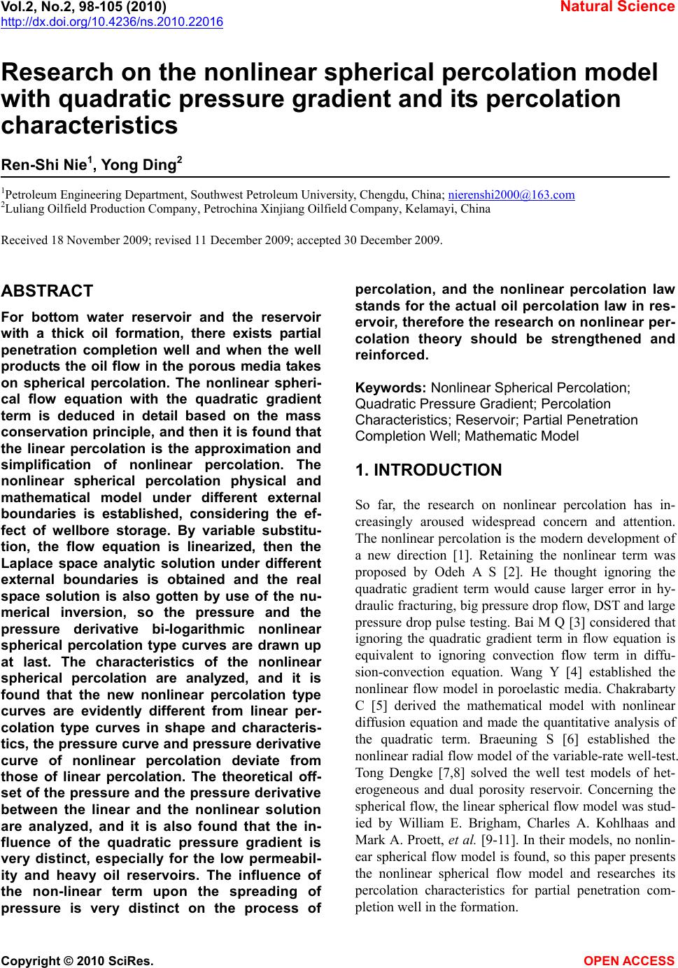Vol.2, No.2, 98-105 (2010) Natural Science
http://dx.doi.org/10.4236/ns.2010.22016
Research on the nonlinear spherical percolation model
with quadratic pressure gradient and its percolation
characteristics
Ren-Shi Nie1, Yong Ding2
1Petroleum Engineering Department, Southwest Petroleum University, Chengdu, China;
2Luliang Oilfield Production Company, Petrochina Xinjiang Oilfield Company, Kelamayi, China
Received 18 November 2009; revised 11 December 2009; accepted 30 December 2009.
ABSTRACT
For bottom water reservoir and the reservoir
with a thick oil formation, there exists partial
penetration completion well and when the well
products the oil flow in the porous media takes
on spherical percolation. The nonlinear spheri-
cal flow equation with the quadratic gradient
term is deduced in detail based on the mass
conservation principle, and then it is found that
the linear percolation is the approximation and
simplification of nonlinear percolation. The
nonlinear spherical percolation physical and
mathematical model under different external
boundaries is established, considering the ef-
fect of wellbore storage. By variable substitu-
tion, the flow equation is linearized, then the
Laplace space analytic solution under different
external boundaries is obtained and the real
space solution is also gotten by use of the nu-
merical inversion, so the pressure and the
pressure derivative bi-logarithmic nonlinear
spherical percolation type curves are drawn up
at last. The characteristics of the nonlinear
spherical percolation are analyzed, and it is
found that the new nonlinear percolation type
curves are evidently different from linear per-
colation type curves in shape and characteris-
tics, the pressure curve and pressure derivative
curve of nonlinear percolation deviate from
those of linear percolation. The theoretical off-
set of the pressure and the pressure derivative
between the linear and the nonlinear solution
are analyzed, and it is also found that the in-
fluence of the quadratic pressure gradient is
very distinct, especially for the low permeabil-
ity and heavy oil reservoirs. The influence of
the non-linear term upon the spreading of
pressure is very distinct on the process of
percolation, and the nonlinear percolation law
stands for the actual oil percolation law in res-
ervoir, therefore the research on nonlinear per-
colation theory should be strengthened and
reinforced.
Keywords: Nonlinear Spherical Percolation;
Quadratic Pressure Gradient; Percolation
Characteristics; Reservoir; Partial Penetration
Completion Well; Mathematic Model
1. INTRODUCTION
So far, the research on nonlinear percolation has in-
creasingly aroused widespread concern and attention.
The nonlinear percolation is the modern development of
a new direction [1]. Retaining the nonlinear term was
proposed by Odeh A S [2]. He thought ignoring the
quadratic gradient term would cause larger error in hy-
draulic fracturing, big pressure drop flow, DST and large
pressure drop pulse testing. Bai M Q [3] considered that
ignoring the quadratic gradient term in flow equation is
equivalent to ignoring convection flow term in diffu-
sion-convection equation. Wang Y [4] established the
nonlinear flow model in poroelastic media. Chakrabarty
C [5] derived the mathematical model with nonlinear
diffusion equation and made the quantitative analysis of
the quadratic term. Braeuning S [6] established the
nonlinear radial flow model of the variable-rate well-test.
Tong Dengke [7,8] solved the well test models of het-
erogeneous and dual porosity reservoir. Concerning the
spherical flow, the linear spherical flow model was stud-
ied by William E. Brigham, Charles A. Kohlhaas and
Mark A. Proett, et al. [9-11]. In their models, no nonlin-
ear spherical flow model is found, so this paper presents
the nonlinear spherical flow model and researches its
percolation characteristics for partial penetration com-
pletion well in the formation.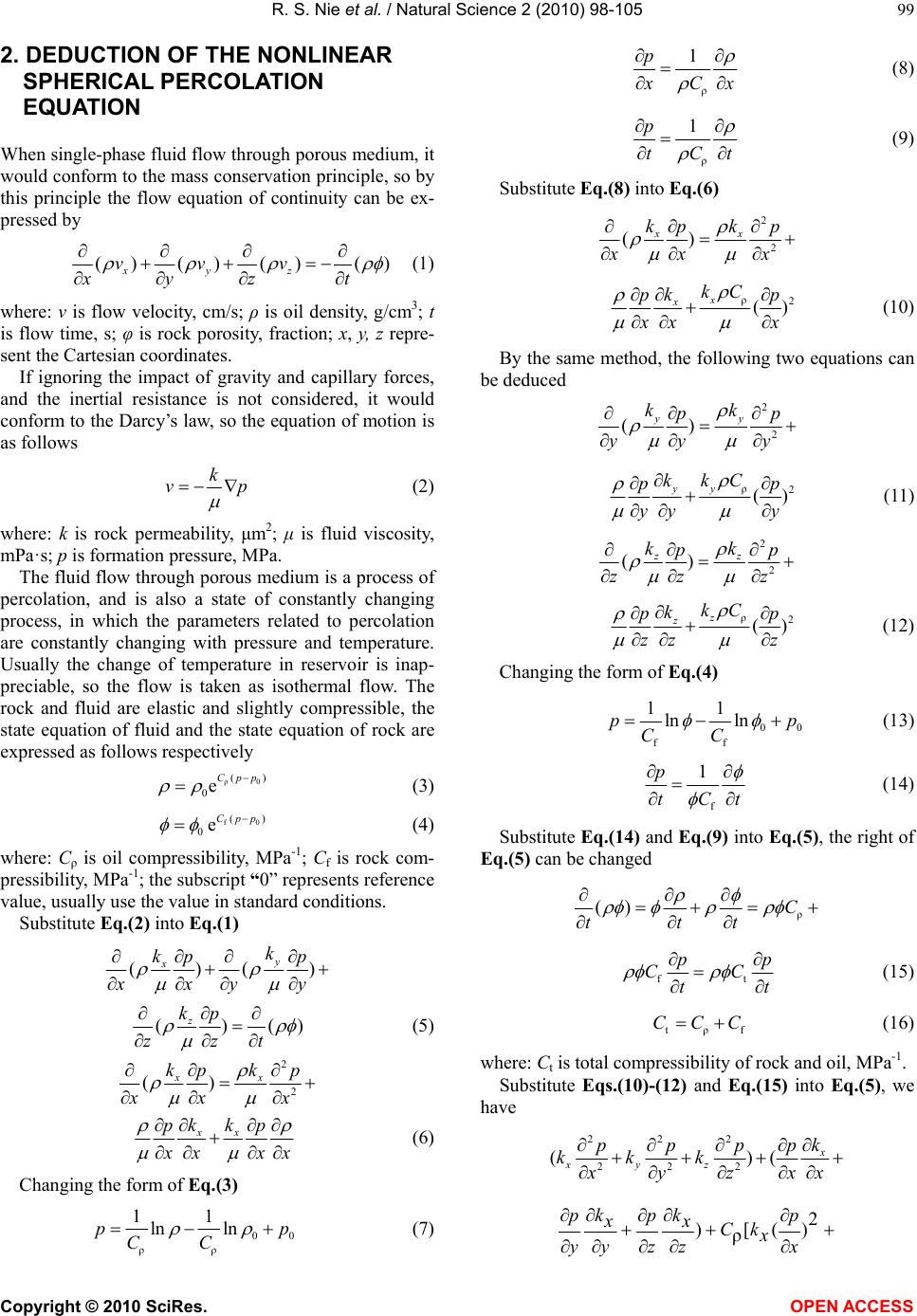

R. S. Nie et al. / Natural Science 2 (2010) 98-105
99
2. DEDUCTION OF THE NONLINEAR
SPHERICAL PERCOLATION
EQUATION
When single-phase fluid flow through porous medium, it
would conform to the mass conservation principle, so by
this principle the flow equation of continuity can be ex-
pressed by
()() ()()
xyz
vvv
xyz t

 
 

 
(1)
where: v is flow velocity, cm/s; ρ is oil density, g/cm3; t
is flow time, s; φ is rock porosity, fraction; x, y, z repre-
sent the Cartesian coordinates.
If ignoring the impact of gravity and capillary forces,
and the inertial resistance is not considered, it would
conform to the Darcy’s law, so the equation of motion is
as follows
k
vp

 (2)
where: k is rock permeability, μm2; μ is fluid viscosity,
mPa· s ; p is formation pressure, MPa.
The fluid flow through porous medium is a process of
percolation, and is also a state of constantly changing
process, in which the parameters related to percolation
are constantly changing with pressure and temperature.
Usually the change of temperature in reservoir is inap-
preciable, so the flow is taken as isothermal flow. The
rock and fluid are elastic and slightly compressible, the
state equation of fluid and the state equation of rock are
expressed as follows respectively
ρ0
()
0eCpp


 (3)
f0
()
0eCpp


 (4)
where: Cρ is oil compressibility, MPa-1; Cf is rock com-
pressibility, MPa-1; the subscript “0” represents reference
value, usually use the value in standard conditions.
Substitute Eq.(2) into Eq.(1)
()()
y
xk
kpp
x
xy y




 
()()
z
kp
zzt






(5)
2
2
()
xx
kk pp
xx
x


 

 
xx
kk
pp
x
xxx






  (6)
Changing the form of Eq.(3 )
00
ρρ
11
ln ln pp
CC
   (7)
ρ
1p
x
Cx






 (8)
ρ
1p
tCt






 (9)
Substitute Eq.(8) into Eq.(6)
2
2
()
xx
kk pp
xx
x


 

 
ρ2
()
x
xkC
k pp
x
xx









(10)
By the same method, the following two equations can
be deduced
2
2
()
yy
kk
pp
yy y


 

 
ρ2
()
yy
kkC
pp
yy y









(11)
2
2
()
zz
kk pp
zz z


 

 
ρ2
()
z
zkC
k
pp
zz z









(12)
Changing the form of Eq.(4)
00
ff
11
ln ln pp
CC


 (13)
f
1p
tCt






 (14)
Substitute Eq.(1 4) and Eq.(9) in to Eq.(5), the right of
Eq.(5) can be changed
ρ
() C
ttt

 


 

ft
pp
CC
tt
 




 (15)
tρf
CCC

 (16)
where: Ct is total compressibility of rock and oil, MPa-1.
Substitute Eqs.(10)-(12) and Eq.(15) into Eq. (5 ), we
have
222
222
()(
x
xyz
k pppp
kkk
x
x xyz






2
)[()
ρ
kk pp p
xx
Ck
x
yy zzx
  


 

R. S. Nie et al. / Natural Science 2 (2010) 98-105
100
22
t
() ()]
yz
pp p
kk C
yz t

 

 
(17)
If the permeability is isotropic and constant,
/0,/0,/0
xyy
kr kr kr, the Eq.(17) be-
comes
222
2
ρ
222
()[()
ppp p
Cx
xyz
 
 
 
22 t
() ()]C
pp p
yz kt

 

 
(18)
Eq.(18) is the governing differential equation in Car-
tesian coordinates, the equation in radial spherical coor-
dinates becomes
22
t
ρ
2
1()() C pp p
rC
rrr ktr

 

 
(19)
where, r represents the radial spherical coordinates.
Eq.(19) is the nonlinear flow governing partial dif-
ferential equation with quadratic pressure gradient term.
We call the second power of the pressure gradient as
quadratic pressure gradient.
The function exp(x) by use of Maclaurin series expan-
sion is written by
2
exp()1/ 2/!
n
xxx xn  (20)
If we use Maclaurin series expansion for Eqs.(3) and
(4) and neglect the second order and the above higher
order item, the Eqs.(3) and (4) can be rewritten by Eqs.
(21) and (22) respectively
0ρ0
[1 ()]Cp p

  (21)
0f 0
[1 ()]Cpp

  (22)
The appearance of quadratic pressure gradient term is
simply because that we didn’t make any simplification
for the state Eqs. (3) and (4) in the deduction of the flow
governing partial differential equation. If we use Eqs.
(21) and (22), instead of Eqs.(3) and (4), in the deduc-
tion of the flow governing partial differential equation,
the quadratic pressure gradient term will not come up,
and the deduced flow equation is the conventional linear
flow equation, which is shown in almost any percolation
mechanics books and papers, so the deduction of the
linear flow equation is certainly omitted here. Owing to
the existence of quadratic pressure gradient, the flow
equation takes on nonlinear properties. Therefore it can
be safely concluded that the conventional linear flow
equation is the approximation and simplification of
nonlinear flow equation with quadratic pressure gradient
term, and that the nonlinear percolation law stands for
the actual flow law of oil in reservoir.
3 .SPHERICAL PERCOLATION MODELS
AND ITS SOLUTION
3.1. Physical Model
For bottom water reservoir, the position of drilling and
completion of oil well is usually in the top of the oil
formation, the flow diagram shown in Figure 1. For
some reservoirs, the oil formation is very thick, the posi-
tion of drilling and completion of well is usually in the
middle of the formation, the flow diagram shown in
Figure 2. For the two actual situations, the oil flow in
the porous media is in the form of spherical percolation.
Physical model assumptions are as follows:
1) A single well with partial penetration completion in
the formation like Figure 1 or Figure 2 products at con-
stant rate, the external boundary may be infinite or
closed or constant pressure;
2) The rock and the single-phase fluid are slightly
compressible, a constant compressibility;
3) Isothermal and Darcy flow, the permeability and
porosity of isotropic properties;
r
w
r
sw
p
e
r
e
h
b
p
sw
Well
Formation
Figure 1. Spherical flow diagram for well completion posi-
tion in the top of the formation.
b
h r
sw
p
w
Well
Formation
Figure 2. Spherical flow diagram for well completion posi-
tion in the middle of the formation.

R. S. Nie et al. / Natural Science 2 (2010) 98-105
101
4) Considering wellbore storage effects (in the begin-
ning of opening well, the fluid stored in the wellbore
starts to flow, the oil in the formation does not flow);
5) At time t=0, pressure is uniformly distributed in the
reservoir, equal to the initial pressure pi;
6) Ignoring the impact of gravity and capillary forces.
3.2. Mathematic Model
The governing differential equation in radial spherical
coordinate system
22 t
ρ
2
1()()
3.6
C
pp p
rC
rr rktr

 

 
(23)
where: r is the radial spherical distance from well, m; the
unit of well production time (t) becomes “h”, so the co-
efficient “3.6” appears in the Eq.(23).
Initial conditions
0it
pp
 (24)
where, pi is initial formation pressure, MPa.
Inner boundary condition
sw
23
()0.921 10
rr
kp
rqB
r 




s
d
0.022105 d
w
p
Ct (25)
where: the rws is called the pseudo well radius of radial
spherical flow, and rws=b/(2ln(b/rw)) [12], b is the forma-
tion penetration thickness of well completion, m; r
w is
the real well radius m; q is oil rate at wellhead, m3/d; B
is oil volume factor, dimensionless; Cs is wellbore stor-
age coefficient, m3/MPa; pw is wellbore pressure, MPa.
External boundary condition
i
lim (infinite)
rpp   (26)
ei (constant pressure)
rr
pp
 (27)
e0 (closed)
rr
p
r

 (28)
where, re is external boundary radius, m.
3.3. Solution to Mathematic Model
The dimensionless definitions are as follows:
Dimensionless pressure

3
Dswi / (0.92110)pkrppqB


 ;
Dimensionless radius based on pseudo spherical flow
radius Dsw /rrr;
Dimensionless wellbore storage coefficient
3
Ds tsw
/ (3.1416)CC Cr  ;
Dimensionless time 2
Dtsw
3.6/()tktCr  ;
Dimensionless quadratic pressure gradient coefficient
3
ρsw
0.92110/ ()qB Ckr 


The dimensionless model is as follows:
The governing differential equation in radial spherical
coordinate system
2
2 DDDD
2
DDD DD
2()
pppp
rrr tr



 

 (29)
Initial conditions
D
D0
0
t
p (30)
Inner boundary condition
D
wD D
DD1
DD
d()1
dr
pp
Cr
tr




 (31)
External boundary condition
D
DDD
lim(,)0 (infinite)
rprt   (32)
DeD
D0 (constant pressure) rr
p (33)
eD
D
D
0 (closed)
rr
p
r

 (34)
Take
D
1lnpx

 (35)
where, x is substitution variable between variables.
Making the upper variable substitutions for Eqs.
(29-34), the model can be converted to
The governing differential equation
2
2
DD DD
2
()
x
xx
rr tr




 (36)
Initial conditions
D01
t
x (37)
Inner boundary condition
D
D1
DD
()0
r
xx
Cx
tr





 (38)
External boundary condition
D
DD
lim(,)1 (infinite)
rxr t   (39)
DeD 1 (constant pressure)
rr
x (40)
DeD
D
0 (closed)
rr
x
r

 (41)
Take

R. S. Nie et al. / Natural Science 2 (2010) 98-105
102
D
/1xyr (42)
where, y is substitution variable between variables.
Making the upper variable substitutions for Eqs.
(36-41), the model can be converted to
The governing differential equation
2
2
DD
yy
tr



 (43)
Initial conditions
D00
t
y

(44)
Inner boundary condition
D
D1
DD
[(1)]
r
yy
Cy
tr



 
 (45)
External boundary condition
D
lim0 (infinite)
ry   (46)
DeD 0 (constant pressure)
rr
y (47)
DeD
DD
1
()0 (closed)
rr
yy
rr


 (48)
Introduce the Laplace transform based on tD, that is
D
DDDD D D
0
[()]()()e d
zt
Lp tpzp tt



 (49)
where, z is Laplace space variable.
So, making the Laplace transform of Eqs.(43-48), the
model becomes:
The governing differential equation in Laplace space
2
2
D
d0
d
yzy
r
(50)
Inner boundary condition in Laplace space
D
D1
D
d
[(1) ]
dr
y
Czy rz



  (51)
External boundary condition in Laplace space
D
lim0 (infinite)
ry   (52)
DeD 0 (constant pressure)
rr
y (53)
DeD
DD
1
()0 (closed)
rr
yy
rr


 (54)
The general solution of Eq.(50) can be expressed by
DD
ee
z
rzr
yA B

 (55)
For infinite boundary:
Substitute Eq.(55) into Eq.(52), have
0A (56)
So the general solution of Eq.(50) becomes
D
e
z
r
yB

 (57)
Substitute Eq.(57) into Eq.(51), have
D
(1)e
z
B
zC zz



  (58)
The general solution of Eq.(50) can be got by
D
D
e
(1)e
z
r
z
y
zC zz




  (59)
At the wellbore bottom, r=rw, rD=1, p=pw, pD=pwD,
x=xw, y=yw, therefore, the solution of the spherical per-
colation model with infinite external boundary in
Laplace space can be got by
D1
w
D
(1)
r
yy zCzz



 (60)
The real space solution yw and the derivative (dyw/dtD)
can be easily obtained by use of Stehfest numerical in-
version [13] for Eq.(60). Substitute the values of inver-
sion into variable substitution relationships, Eq.(35) and
Eq.(42), so the real space solution pwD and the derivative
(dpwD/dtD) can be certainly gained. Accordingly, the
pressure and the pressure derivative bi-logarithmic type
curves of nonlinear spherical percolation can be drawn
up (see Figure 3).
For constant pressure boundary:
At the wellbore bottom rD=1, y=yw, the Eq.(55) be-
comes
w
ee 0
zz
ABy


 (61)
Substitute Eq.(61) into Eq.(51) and Eq.(53), have
respectively
ee
zz
zAz B


 
Dw
(1)Czy z



 (62)
Figure 3. Type curves of nonlinear spherical percolation af-
fected by β under infinite external boundary.

R. S. Nie et al. / Natural Science 2 (2010) 98-105
103
eD eD
ee 0
zr zr
AB

  (63)
For closed boundary:
Substitute Eq.(61) into Eq.(54), have
eD eD
eD eD
(1)e(1)e 0
zr zr
zrA zrB

  (64)
Combining Eqs.(61-64) , the coefficients A and B and
the function at wellbore w
y
in Laplace space can be
easily obtained by use of some linear algebra method
(such as Gauss-Jordan reduction, etc), then nonlinear
spherical percolation type curves can also be drawn up
(see Figure 4 and Figure 5) by use of the same method.
4. CHARACTERISTICS OF THE
NONLINEAR PERCOLATION
4.1. Parameter Sensitivity Analysis to Type
Curves
Figure 3 shows the type curves of nonlinear spherical
percolation affected by β under infinite external bound-
ary. Can be seen from the figure, the curves vary with
the value of the dimensionless quadratic pressure gradi-
ent coefficient β (from up to down, β=0, 0.2, 0.4), when
β=0 it is just the curve of linear percolation model. It can
be easily seen that the curves have the trait of unit slope
in the wellbore storage stage, which shows that there is
no influence of quadratic pressure gradient in this flow
stage, and that the location of the pressure and the pres-
sure derivative curves is lower than that of the conven-
tional linear model curve in the stage of infinite-acting
radial spherical flow. The bigger the β is, the greater the
offset is.
Figure 4 and Figure 5 show the type curves of
nonlinear spherical percolation affected by β under con-
stant pressure external boundary and closed external
boundary respectively. Can be seen from the figures, the
trait of unit slope in the wellbore storage stage still exist
and there still exists a offset due to the effect of β, but in
the late flow stage of boundary response the pressure
derivative curves is going down until focusing on a point
for constant pressure boundary and the pressure deriva-
tive curves is going up until focusing on a line together
with the pressure curves for closed boundary, which is
completely different from Figure 1.
Figure 6 shows the type curves of nonlinear spherical
percolation affected by CD under infinite external
boundary. Can be seen from the figure, the curves vary
with the value of the dimensionless wellbore storage
coefficient CD, and the bigger the CD is, the lower
thepressure derivative curve is. Figure 7 shows the type
curves of nonlinear spherical percolation affected by reD
under different external boundaries. Can be seen from
the figure, the curves vary with the value of the dimen-
Figure 4. Type curves of nonlinear spherical percolation af-
fected by β under constant pressure external boundary.
Figure 5. Type curves of nonlinear spherical percolation af-
fected by β under closed external boundary.
Figure 6. Type curves of nonlinear spherical percolation af-
fected by CD.
sionless radial spherical radius reD, and the bigger the reD
is, the later the time of going up or going down is.
According to the definition of β and the probable val-
ues of β (Table 1), it is clearly demonstrated that β is
proportional to oil viscosity μ, and inversely proportional
to formation permeability k. So there is usually a bigger
β for the low permeability, heavy oil reservoirs, and the
influence of the quadratic pressure gradient nonlinear
term is very distinct, the quadratic pressure gradient
should not be neglected. For the fixed group of parame-
ters (q, B, Cρ), the speed of pressure wave propagation

R. S. Nie et al. / Natural Science 2 (2010) 98-105
104
Figure 7. Type curves of nonlinear spherical percolation af-
fected by reD.
Table 1. The probable values of β.
k/(×10-3μm2) μ/(mPa·s) β
100 25 0.0058
10 25 0.0580
1 25 0.5800
100 100 0.0230
10 100 0.2300
1 100 2.3000
becomes slower when k/μ decreases with the increasing
of β. Compared with the conventional linear model,
given a fixed production time, pressure decline slows
down and the speed of decline is inversely proportional
to β, which is completely accordant with the theoretical
curves as Figures 3-5. In conclusion, for a concrete res-
ervoir, due to the effect of quadratic pressure gradient,
compared with conventional linear model, the time of
stable production of the nonlinear model is prolonged on
condition that the same decline of reservoir pressure.
4.2. The Influence Analysis of Nonlinear Term
Table 2 and Table 3 exhibit the results of the pressure
offset and pressure derivative offset analyses vs. Figure
3. As shown the data in these tables, the offset increase
with the increasing of time at a constant β, and pressure
derivative relative offset is greater than the pressure rela-
tive offset at a fixed time. From the data in the table, it is
found that the impact of the quadratic gradient is ex-
tremely intense when time is particularly long and the
quadratic coefficient β is particularly large, so the quad-
ratic pressure gradient should be retained in flow equa-
tion. After all, the nonlinear percolation law is the actual
flow law of oil in porous medium, so the research on the
nonlinear percolation model and its percolation law with
quadratic pressure gradient should be strengthened and
reinforced.
5. CONCLUSIONS
In this paper it is demonstrated that the quadratic pres-
sure gradient has some distinct influence on the well-
bore1) The linear percolation is the approximation and
simplification of nonlinear percolation with quadratic
pressure gradient term.
Table 2. The offset analysis of nonlinear term(β＝0.2).
PwD P’wD·tD/CD
tD/CD
linear nonlinear
offset relative
offset /% linear nonlinear
offset relative
offset /%
102 0.943292 0.864578 0.078714 8.34 0.029071 0.024059 0.005012 17.24
103 0.982148 0.896753 0.085395 8.69 0.008939 0.007390 0.001549 17.33
104 0.994357 0.906908 0.087449 8.79 0.002804 0.002312 0.000492 17.55
105 0.998216 0.910121 0.088095 8.83 0.000886 0.000728 0.000158 17.83
Table 3. The offset analysis of nonlinear term(β＝0.4).
PwD P’wD·tD/CD
tD/CD
linear nonlinear
offset relative
offset /% linear nonlinear
offset relative
offset /%
102 0.943292 0.801013 0.142279 15.08 0.029071 0.020499 0.008572 29.49
103 0.982148 0.828462 0.153686 15.65 0.008939 0.006302 0.002637 29.50
104 0.994357 0.837153 0.157204 15.81 0.002804 0.001970 0.000834 29.74
105 0.998216 0.839906 0.158310 15.86 0.000886 0.000622 0.000264 29.80

R. S. Nie et al. / Natural Science 2 (2010) 98-105
105
2) The new-style type curves of nonlinear spherical
percolation with quadratic pressure gradient effect in
shape and characteristics are obviously different from
the type curves of linear model, the location of the pres-
sure and the pressure derivative curves is lower than that
of the conventional linear model curve.
3) The type curves are affected by the quadratic gra-
dient coefficient β, the offset of pressure and pressure
derivative is directly proportional to β and time.
4) For a concrete reservoir, due to the effect of quad-
ratic pressure gradient, compared with conventional lin-
ear model, the time of stable production of the nonlinear
model is prolonged on condition that the same decline of
reservoir pressure.
5) The impact of the quadratic pressure gradient under
certain conditions is extremely intense, especially for the
low permeability and heavy oil reservoirs, and the quad-
ratic pressure gradient term should not be neglected and
should be retained in flow equation.
6) The nonlinear percolation law is the actual flow
law of oil in porous medium, so the research on the
nonlinear flow model and its application with quadratic
pressure gradient should be strengthened and reinforced.
REFERENCES
[1] Yan, B.S. and Ge, J.L. (2003) New advances of modern
reservoir and fluid flow in porous media. Journal of
Southwest Petroleum Institute, 25(1), 29-32, (in Chi-
nese).
[2] Odeh, A.S and Babu, D.K. (1998) Comprising of solu-
tions for the nonlinear and linearized diffusion equations.
SPE Reservoir Engineering, 3(4), 1202-1206.
[3] Bai, M.Q. and Roegiers, J.C. (1994) A nonlinear dual
porosity model. Appl Math Moclellin, 18(9), 602-610.
[4] Wang, Y. and Dusseault, M.B. (1991) The effect of quad-
ratic gradient terms on the borehole solution in poroelas-
tic media. Water Resource Research, 27(12), 3215-3223.
[5] Chakrabarty, C., Farouq, A.S.M. and Tortike, W.S. (1993)
Analytical solutions for radial pressure distribution in-
cluding the effects of the quadratic gradient term. Water
Resource Research, 29(4), 1171-1177.
[6] Braeuning, S., Jelmert, T.A. and Sven, A.V. (1998) The
effect of the quadratic gradient term on variable-rate
well-tests, Journal of Petroleum Science and Engineering,
21(2), 203-222.
[7] Tong, D.K. (2003) The fluid mechanics of nonlinear flow
in porous media. Beijing: Petroleum Industry Press in
Chinese, (in Chinese).
[8] Tong, D.K., Zhang, Q.H. and Wang, R.H. (2005) Exact
solution and its behavior characteristic of the nonlinear
dual-porosity model. Applied Mathematic and Mechanics,
26(10), 1161-1167, (in Chinese).
[9] William, E.B., James, M. and Peden, K.F.N. (1980) The
analysis of spherical flow with wellbore storage. SPE
9294.
[10] Charles, A.K. and William, A.A. (1982) Application of
linear spherical flow analysis techniques to field prob-
lems-case studies. SPE 11088.
[11] Mark, A. and Proett, W.C.C. (1998) New exact spherical
flow solution with storage and skin for early-time inter-
pretation with applications to wireline formation and
early-evaluation drillstem testing. SPE 49140.
[12] Joseph, J.A. and Koederitz, L.F. (1985) Unsready-state
spherical flow with storage and skin. SPEJ, 25(6),
804-822.
[13] Stehfest H. (1970) Numerical inversion of Laplace
transform algorithm 368, Communication of the ACM,
13(1), 47-49.