F. Liu et al. / J. Biomedical Science and Engineering 3 (2010) 217-220
Copyright © 2010 SciRes.
219
JBiSE
ous column bicluster B'(I',J'), which allows II' and
J J', or I I' and J J'. According to Cheng
&Church’s greedy algorithm [9], for any given bicluster
B(I,J), the MSR of new bicluster B’(I∪R,J) will not ex-
pand, where R stands for a row set as follows:
}),()(
||
1
;{ 2
Jj
IJIjiJij JIMSRaaaa
J
IiR
So this greedy method can be adopted in adding some
rows into the bicluster as Algorithm 2 shows:
Algorithm 2: Greedy Expanding
Input: M(R,C), a transformed genes expression matrix of size s
×q, and there are k primary clusters
Output: k primary clusters
Iteration:
Step1: Initialize each cluster C
i
(1≤i≤k)
Step2: Compute the set of columns Q={q
1
,q
2
,…,q
m
} which
not belongs to any of the primary cluster.
Step2.1: Compute the MSR score if row j (j∈Q) is added to
cluster C
i
.
Step 2.2: Add the row with the least MSR into cluster C
i
,
and delete it from set Q
Step 2.3: Compute the MSR of C
i
and go to step 2 if it is less
than δ.
Step 3: Go to Step1 to calculate the next cluster until all the
primary clusters are calculated.
Step7: output the k primary clusters
4.1.2.3. Rapid Expansion of Classification
However, the algorithm above repeats Step2~Step5 too
frequently. Thus, we improve the algorithm based on the
Greedy Principle.
Firstly, scoring the primary cluster B(I,J) with α, and
the largest cluster B'(I',J') with δ. If the count of the steps
is no more than k, the increment of each step will be
(δ–α)/k. Thus, the increment to the cluster of adding
each row should be no more than (δ–α)/k. And then, an
improved algorithm will be introduced:
Algorithm 3: Rapid expansion of classification
Input: M(R,C), a transformed genes expression matrix of size s
×q, and there are k primary clusters
Output: k clusters
Iteration:
Step1: Initialize each cluster C
i
(1≤i≤k)
Step2: Compute the set of columns Q={q
1
, q
2
,…,q
m
} which
not belongs to any of the primary cluster.
Step3: For each row j in Q and each cluster C
i
.
Step 3.1 Calculate MSR score if row j is added to cluster C
i
.
Step 3.2: Add the rows into each cluster C
i
if their MSR score
is less than (
δ
-
α
)/r.
Step 3.3 Delete the rows from set Q
Step 3.4: Recompute the MSR of C
i
, and go to Step 3 if
their score is less than δ and Q is not null.
Step 4: Delete several rows to make each bicluster’s score
less than
δ
by the algorithm proposed by Cheng & Church.
Step5: Print out the k clusters
4.1.3. Phase 3: Generation of the Sequential δ-cluster
In this phase, the time-lagged bicluster the is extracted
from δ-clusters.
Firstly, assuming I={r1,r2,…,rp} as a set of the rows
of δ-cluster B(I,J). There ri represents the ith row in
M(R,C). Secondly, assume that G={g1,g2,…,gn} is the
gene set of original expression matrix X(G,T). Set
T={ct1,ct2,…,ctm}, and q is the number of sequential
points of M(R,C). There /
i
rm
mod
i
r
represents the gene at
row i of δ-cluster, and m
is the start time.
Then the target bicluster B (I’, S, q) will be got.
4.1.4. The Overall Algorithm:
Generally, q is a positive integer within 100, and we
enumerate all possible q. The overall algorithm is:
Algorithm 4: the overall algorithm
Input: Gene expression matrix X(G,C) with m rows and n
columns, threshold α、δ and q.
Output: the best time-lagged bicluster.
Iteration:
Ste p1 : For each different q
Ste p1 . 1: Transform the matrix to M(R,C)
Ste p1 . 2:Find the k-best primary cluster using Algorithm 1.
Ste p1 . 3:Expand the clusters using Algorithm 3.
Ste p1 . 4:Print out the k best clusters and transform them into
sequential δ-clusters
Step1.5: Go to step 1 until all the q is considered.
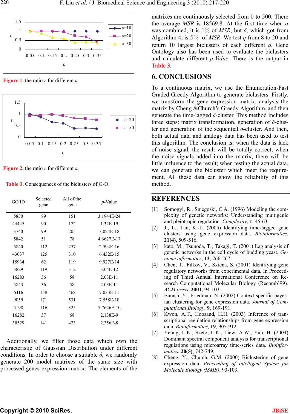
5. EXPERIMENTS AND RESULTS
Firstly, we randomly generate a 200×20 matrix X(G,T)
of positive continuous within 100. Secondly, randomly
generate a k*s bicluster B(I,J). At last, replace several
rows in X(G,T) by lines of B(I,J) at random points.
If set α=0.2、δ=1、k=4 、4≤q≤20, and the size of B(I,J)
is between 5×5~200×20. The algorithm can efficiently
find the implanted bicluster.
Additionally, we also add some noise into the matrix.
Selecting ε|I||J| data from B(I,J) and adding a value be-
tween –a to a to this matrix. Let k be the quantity of the
output of bicluster and each of them is denoted by
Bk(Ik’,Jk’). Accuracy r can be calculated as the over-
lapped part of Bi(Ii’,Ji’) and B(I,J) as follows:
|'|*|
|'|*|
'|
ii
ii
'|
IJJ
r
IJJ
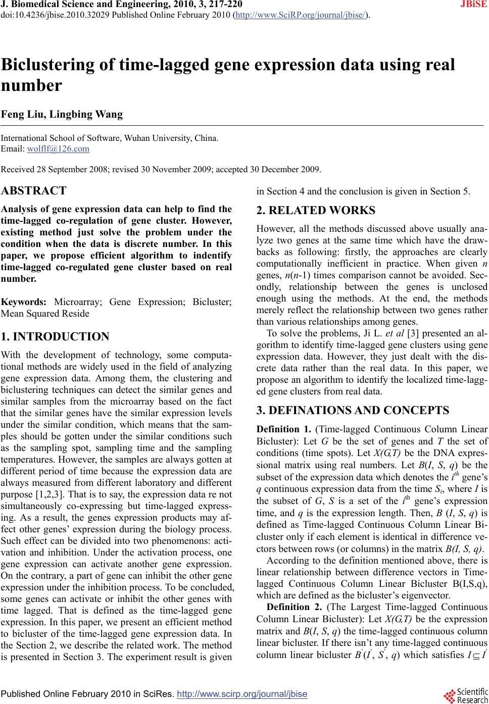
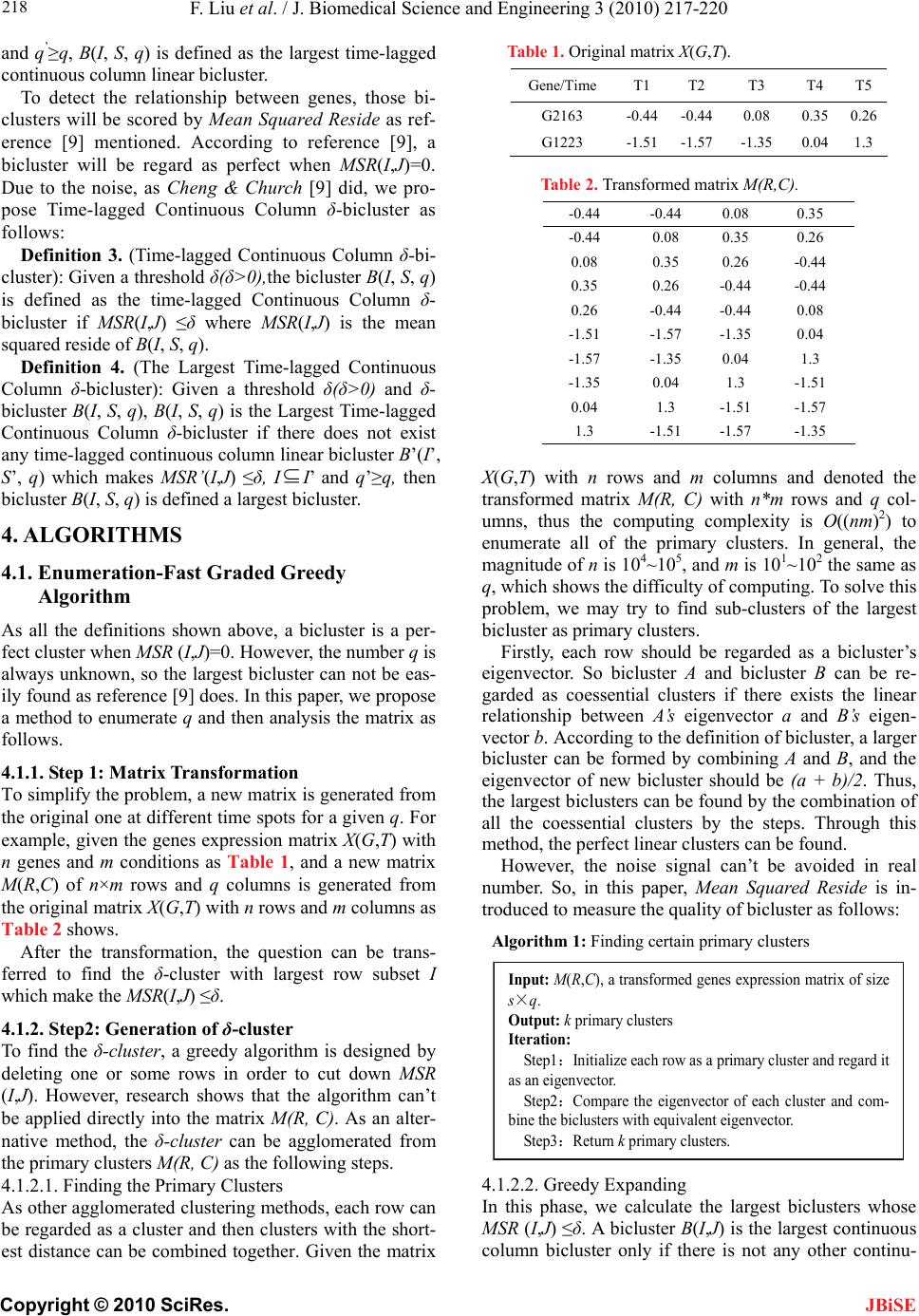
If set α=2、δ=20, the ratio r with different a, ε is
following:
Figure 1 has shown that the more noise, the worse the
result will be. And the stronger noise, the worse the re-
sult will be. Under the condition with a few noises, the
result is acceptable.
Figure 2 The parameter δ should be increased to im-
prove the algorithm if the noise signal is too strong.