Intelligent Control and Automation
Vol. 4 No. 1 (2013) , Article ID: 27848 , 8 pages DOI:10.4236/ica.2013.41013
An Enhanced Genetic Programming Algorithm for Optimal Controller Design
1Isra University, Amman, Jordan
2University of Technology, Baghdad, Iraq
Email: rami.maher@iu.edu.jo, moh62moh@yahoo.com
Received August 16, 2012; revised September 22, 2012; accepted September 30, 2012
Keywords: Genetic Programming; Optimal Control; Nonlinear Control System
ABSTRACT
This paper proposes a Genetic Programming based algorithm that can be used to design optimal controllers. The proposed algorithm will be named a Multiple Basis Function Genetic Programming (MBFGP). Herein, the main ideas concerning the initial population, the tree structure, genetic operations, and other proposed non-genetic operations are discussed in details. An optimization algorithm called numeric constant mutation is embedded to strengthen the search for the optimal solutions. The results of solving the optimal control for linear as well as nonlinear systems show the feasibility and effectiveness of the proposed MBFGP as compared to the optimal solutions which are based on numerical methods. Furthermore, this algorithm enriches the set of suboptimal state feedback controllers to include controllers that have product time-state terms.
1. Introduction
Genetic Programming (GP) is a stochastic search method that inspired by the selection and the natural genetics. GP is characterized by its capability to evolve models (structure as well as parameters) for different kinds of problems in different scientific fields. However, GP in its basic standard form needs to be revised according to the applications nature and requirements. In order to increase the efficiency of GP to deal with optimal control problems, a set of syntactic rules are created to force all tree structures in the population such that the GP will evolve only solutions of desired form. These rules state for each node which terminal node and non-terminal node can be its children nodes while generating new trees and performing genetic operations. The idea of using constraint syntactic structure GP was suggested by Koza [1]. Then it was extended by Montana, who has developed the idea of strongly typed GP [2]. Further development was announced under what is known as a grammatical GP [3].
In many application areas, the GP is one of the powerful current soft computing algorithms [4-6]. It can solve different types of problems in control discipline. For instance, the GP is recently used to solve the well-known Hamilton-Jacobi-Bellman (HJB) equation. Joe Imae et al., in their works [7,8] showed how GP can be used to solve the HJB equation efficiently for linear and nonlinear control systems. The results of the used examples are coincident that based on the theoretical solutions. Enhancing the standard tree structure used in the GP algorithm by new thoughts, ideas, and tools represent a road map to get an efficient methodology for controller design for nonlinear dynamic systems.
2. The Proposed MBFGP Algorithm
This paper proposes an approach to force GP tree structures to represent a certain random number of basis functions that are linear in parameters. The approach will be called MBFGP. In this way, the search space of all possible GP trees is reduced to a subspace of trees that satisfies the required data type constraints.
These constraints are defined before learning takes place, and they have an impact on the evolutionary process of the algorithm. Three considerations arise when GP is implemented with trees that have such constrained syntactic structures. These considerations are:
1) The initial population of the random individuals must be created such that every program in the population has the required syntactic structure.
2) When the genetic operations are performed, the required syntactic structure must be preserved so that the operations will always produce the offspring conforming to the syntactic structure.
3) The fitness measure must consider the syntactic structure.
The basic parts constituting of the MBFGP and other related details will be explained in the following subsections.
2.1. Representation
The structures of program trees in MBFGP are composed of a random number of linear and/or nonlinear basis functions (terms), which are forced to be linear in parameters. The MBFGP tree structure has a single root node, internal nodes, and leaf nodes. The general tree structure of MBFGP is divided into two main parts: the head part constructed from fixed (restricted to have specific locations in the tree) problem independent nodes set Σ, f or R and the tail part constructed from unfixed (freely to appear in the tree) problem dependent nodes set as shown in Figure 1.
The node Σ is restricted to appear only in the root of the tree structure, so this node will root every program tree. It allocates a space of a specified number Nb of arguments while it is created. However, not all of these arguments will be filled, but instead a random number of them in the range between 1 and Nb will be filled. The rest of the arguments is left empty. These empty argument spaces have an important role through the adaptation process of structures. They may be filled during the implementation of genetic operations on its tree structure.
This property gives the node Σ the ability to have been varying numbers of filled arguments through adaptation, and gives the overall structures high flexibility to adapt their size. The basis function node has two arguments of fixed type; it is also restricted to appear only as a child (argument) of the root node in every tree structure. The two arguments of this node carry different types of nodes. The first argument is restricted to carry only the numeric constant terminal node R, while the second argument may represent any unrestricted node from unfixed terminal and function sets. The R nodes represent the coefficients of the basis functions that are present in the tree structure. Each R node is restricted to appear only in the first argument of each basis function node. Finally, the unfixed node set represents all available functions and terminals that are chosen by the user to appear in the com-
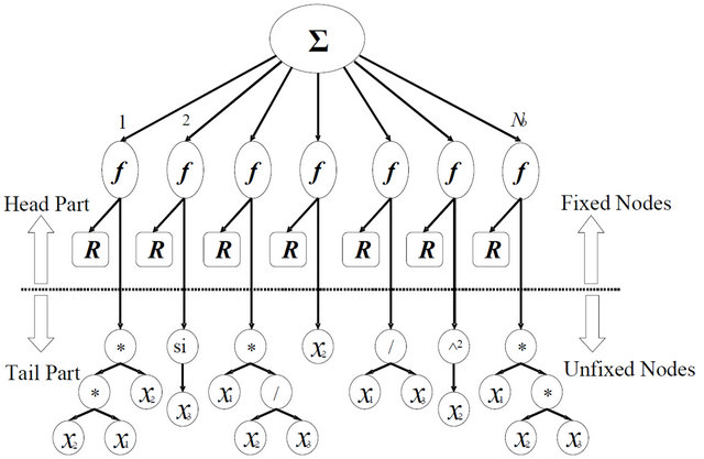
Figure 1. A general tree structure of MBFGP.
puter program.
According to the set of specific rules that are defined to specify which terminals and functions are allowed to be child nodes of every function in the MBFGP tree structure, fixed sequence of nodes for each basis function will appear in the head part. On the other hand, in the tail part, the basis functions are completed freely without any restrictions on the sequence of nodes. Therefore, different basis functions in the tree structure can be obtained.
2.2. Initial Population
The initial population of random tree structures must be created using the syntactic rules of construction. The desired structure of the multiple basis functions can be created merely by restricting the choice of function for the root of the tree to node Σ. Then, using uniform random distribution, a random number is chosen in the range 1 to Nb. This random number specifies the number of arguments of the node Σ that is required to be filled. All branches of the node Σ are restricted to carry the basis function f nodes.
The first argument of each function node f is restricted to carry numeric constant terminal node R. The value for each created numeric constant terminal node is chosen randomly in a specified range (e.g., in range −10 to 10 with step size 0.001). The second argument is unrestricted. It can carry any available function from the set of the unfixed functions or any available terminal from the set of the unfixed terminals. The proceeding nodes in each branch are chosen randomly from the same unfixed function and terminal sets. The end of the tree structure is bounded by the parameter of maximum creation depth; this parameter is determined by the user.
2.3. Genetic Operations
The genetic operations, as is the case with the creation of initial population, must respect the syntactic rules to produce the correct offspring tree structure. The proposed genetic operations for MBFGP are described in what follows.
- Crossover Operation
Two types of crossover operation are implemented on MBFGP tree structures. These types are: the Internal Crossover Operation which occurs in the tail part of each parent tree structure. The operation starts by choosing randomly two parental trees from the population based on fitness measure. Choosing a crossover point in each parent is restricted to picking randomly a node from the tail part in order to preserve the required tree structure for the produced offspring. The simplest way to perform the restraining process is to exclude the fixed nodes (Σ, f and R) of the parental tree from being selected as a crossover point of either parent. This restraining secures that the crossover preserves the syntactic structure, and it will always produce the offspring tree structures. The second type is the External Crossover Operation, which occurs in the head part of the tree structure. In this type, two parental trees are selected randomly from the population based on fitness measure.
The number of existent basis functions in each parental tree is counted. Therefore, the syntactic rules enforce the crossover point in each parent to be one of the basis functions, which are selected randomly from the existent basis functions in the parental tree. Then, the swapping between these two selected basis functions is implemented to produce two new offspring.
- Mutation Operation
Different types of mutation operation are proposed. They are:
1) Swap operation, which is applied to the tail part of the parental tree structure only. The present unfixed nodes (functions and terminals) in the tail part of the selected parental tree structure are counted. One unfixed node is randomly selected from the tree structure. The number of arguments kγ of the selection is checked. Another new node is chosen randomly with kγ arguments from combined sets of unfixed function and terminal nodes. The new chosen node changes the existent node in the tree structure. If one considers the number of arguments of the terminal node is zero, another randomly chosen terminal node can swap the original terminal node.
2) Shrink operation, which is applied similarly as the swap operation. It begins by choosing randomly an unfixed function node and then the chosen function node is deleted and replaced with its child. If the deleted function node has a lot of children, one child among them is chosen randomly to take the place of its parent in the tree, and the rests of the children are deleted. This operation eventually leads to a lower depth of the overall tree.
3) Inverse shrink operation which has two modes of operations: the internal mode operates in the tail part, and the external mode operates in the head part. The internal operation will start by picking randomly an unfixed node. The sub-tree rooted at this node is stored and then deleted from the parental tree. Then, a new function node is chosen randomly from the available set of the unfixed function to take the place of the original unfixed node. The stored sub-tree is inserted back in the first argument of the new node of the unfixed function. If the new function node has more than one argument, randomly created sub-trees fill the remaining arguments. The depth of the created sub-trees is controlled by the parameter of maximum allowable depth. This operation eventually might lead to a higher depth of the overall tree. The external operation works such to increase the number of basis functions in the produced offspring. Nevertheless, the operation is ignored when the number of basis functions in the parental tree is equal to the maximum allowable number Nb. In this case, the offspring is an exact copy of the parent tree.
4) Branch operation which has also two modes of operation, internal and external. The former one works such to create randomly a sub-tree using available unfixed function and terminal sets with respect to the maximum allowable depth. Then, the new created sub-tree is inserted in the mutation point to produce a new offspring. A special case of this operation involves inserting a single terminal node at the selected mutation point. While the external operation works such to create a new subtree rooted with basis function node f. It is created with respect to the syntactic rules of construction, and it is inserted instead of a randomly deleted basis function to produce a new offspring.
- Additional Genetic Operations
Additional proposed operations that are used to vary and adapt the tree structures. They are:
1) Endowment operation: The name “Endowment” has been chosen to indicate the process of basis function endowment that occurs between two individuals. This operation starts by choosing randomly two parental individuals on the base of the fitness. The number of existent basis functions in each parent is counted. One basis function of the existent basis functions in each parent is chosen randomly. A copy of the selected basis function in the first parent is added to the basis functions in the second parent to produce the first offspring. While a copy of the selected basis function in the second parent is added to the basis functions in the first parent to produce the second offspring.
2) Delete operation, which is used to delete a basis function of the individual on the bases of the fitness value.
3) Merging operation: It edits and simplifies the individual tree structure during GP running. For example, if the tree has two or more basis functions with similar internal structure and contents, then this operator merges them in one basis function.
2.4. Enhancement Operations
A number of enhancement operations are proposed here. They are:
1) Nested function operation: It is responsible for solving the problem of the nested mathematical functions in the individual solutions. Every nested mathematical function node in the tree structure is deleted and replaced by a new sub-tree, which is randomly created. This operator works on all the individuals in every generation.
2) Structural Sorting Operation: It emphasizes that the tree structure as well as the fitness of the individual is considered through implementing the sorting. The population of individuals is sorted first according to the fitness measure with the fittest at the top. Then it is starting from the best individual in the sorted population to pick the best individual and put it in a new list. The procedure proceeds to the less fit individual, if its tree structure and components are not picked before. This means that, any individual that has a structure with components being picked before is ignored, and thus each individual tree structure along with its components is picked only once. The new list of sorting will contain different sorted individuals. This structural sorting operation is based on fitness, and at the same time the sorted individuals are of different structures and components.
3) Enrichment Operation: In order not to discard too soon structures that may be valid, the operation uses first the proposed structural sorting operation. Then a specified number of the individuals is retained from the sorted population list. The proposed method feeds the next population by a number of trees that are different in structures and/or components. In this way, it increases the structural diversity in the subsequent generations.
4) Contribution Operation: It determines the contribution of each of the basis functions in the individual. It resolves the problem of poor diversity of the basis functions by deleting any basis function that has a trivial contribution in the fitness measure. The contribution operation is an effective method to determine which basis functions are significant in MBFGP, and are controlled by the frequency parameter Fco. It is either 1, 0, or an integer greater than one, thus the contribution operation is to be applied to every generation, to no generation or with a certain frequency respectively. In the Appendix, the operation algorithm is shown.
5) Numeric Constant Mutation: It is used, during the GP run, for the known reasons of replacing some of the numerical constant node values by new ones in the individual [6]. The proposed MBFGP here applies two proposed modes of mutating numeric constant node values. Before GP run, the user must specify the range and the resolution of the numeric constant node values (e.g., the range is –10 to 10 with resolution of 0.001). In this case, the algorithm avoids the use of default precision of the floating constant valid in the programming language. This gives the algorithm the ability to ignore the least significant digits in the numeric constant value. The number of numeric constant nodes to be mutated in each individual is chosen randomly in the range 1 to n. For example, if the range is 1 to 3, then this will mean that moving in three dimensions on the cost surface of the numeric constant gives a good probability to climb out the local minimum or maximum. Then after the number of numeric constant nodes that will be mutated is determined, these numeric constants are chosen randomly in the tree. Each value of the numeric constant node is randomly chosen according to one of the following methods. The first method suggests that the new numeric constant values are chosen at random from a specific uniform distributed chosen range. The selection range for each numeric constant is specified as the old value of the numeric constant plus or minus a specified a percentage of the total allowed range. Therefore, it lets the mutation operation explore all the search space and avoid falling in local minimum or maximum. The second method suggests selecting the location of the digit to be mutated randomly. The new value of the numeric constant is equal to the old value plus or minus one for the selected digit. For example, if the old value is 3.791 and the least significant digit is chosen as the digit to be mutated, then the new value of the constant will be either 3.792 or 3.790 with equal probability. Therefore, the second method is useful for fine tuning where the need is only for small change in the numeric constant node values.
3. Optimal Control Solution Based MBFGP
As a first test of the proposed MBFGP, the design of controllers for nonlinear dynamic systems is introduced and compared to optimal control solutions. To emphasize the importance of using MBFGP, the systems are chosen such to have the only numerical solution and not a closedform one.
As it is known, with numerical methods, there are many difficulties concerning the accuracy and the convergence of the solution. In such circumstances, it is hoped that GP is a better alternative. Because not only a solution can be found, but also it will provide many possible solutions whose structures can be controlled by the designer. Therefore, based on the accuracy and the simplicity of the implementation, a choice of one solution can be decided later.
To illustrate the use of the MBFGP algorithm for solving optimal problems, three classical examples will be considered. The results are compared to that obtained by conventional optimal control theory.
Example 1
Consider the Van der Pol system given by
 (1)
(1)
It is required to determine the optimal control, which transfers the system to x1(10) = x2(10) = 0, while minimizing the performance index.
 (2)
(2)
In [9], the method of the conjugate gradient is used to obtain the optimal control, where the optimum value is found to be approximately 21.4. However, when the method of control vector parameterization CVP is used, it is shown [10] that the optimum value is 21.4612, and the control law is
 (3)
(3)
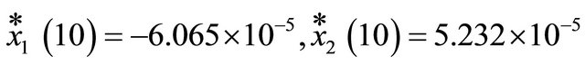
The terminal values of the optimal trajectories are
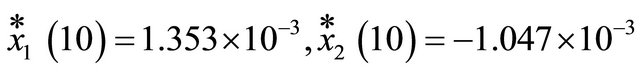
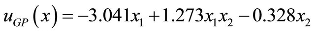
The enhanced algorithm of MBFGP is now used to evolve optimal control laws. The MBFGP is enforced to evolve two forms of control laws. The first one is a function of the time and the system states uGP(x, t) while the second is a function of system states only uGP(x). In the first case, the unfixed terminal set is T = {x1, x2, t, one} while in the second case, the unfixed terminal set is T = {x1, x2, one}. The unfixed function set in both cases is F = {*, /, pow}. The fixed numeric constant node R is in the range −10 to 10 with a resolution of 0.001. A special integer numeric constant node R’ is used to appear only in the power function using special structural constraint rules. The value of this type of numeric constant node is mutated by special type of mutation operation when the pow function is chosen in swap mutation operation. The integer range for R’ node is −5 to 5. The fitness value is calculated discretely with 0.001 step size. At each step, the system equations are integrated numerically to obtain the instantaneous system states.
MBFGP control parameters are illustrated in Table 1, and the results are as follows:
 (4)
(4)
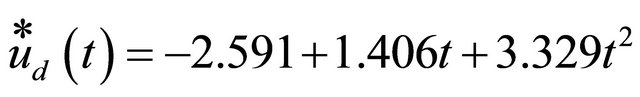
The optimum value is 21.4335, and the terminal trajectory values are
Whereas,
 (5)
(5)
The optimum value is 21.4572 and the terminal trajectory values are
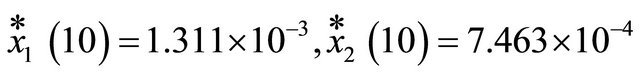
Figure 2 shows the control actions of MBFGP and CVP approaches. As shown, they are all approximately the same. Although the first solution gives less minimal value of J*, the so close results address the second solu
Table 1. GP control parameters (Example 1).
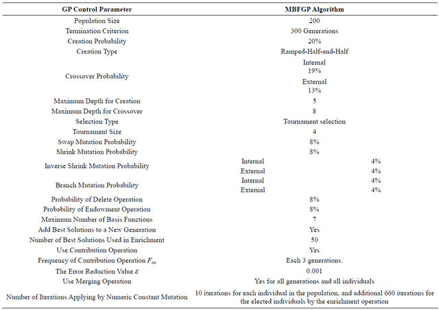
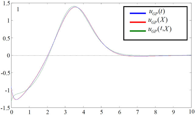
Figure 2. Optimal controls of MBFGP and CVP approach.
tion for the practical implementation. The most interesting results are that GP can result in different controller structures.
Example 2
Consider the following optimal control problem
 (6)
(6)
It is required to find the optimal control law that minimizes the performance index
 (7)
(7)
When the conjugate gradient method is used to solve this problem, it is found that within 17 iterations, the optimum value of the J(u) is 41.5953. Again, when CVP approach is used, the minimum return value J* is equal to 41.596 and the control law as a function of time is given by
 (8)
(8)
The MBFGP algorithm combined with numeric constant mutation operation is proposed to evolve three control laws ,
, 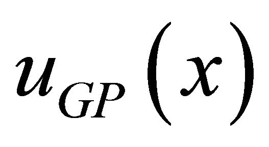 , and
, and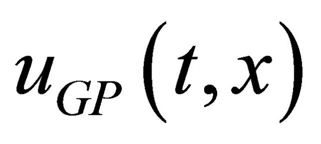 . These different functions of control laws can be obtained by enforcing the unfixed terminal sets in MBFGP algorithm to be T = {t, one}, T = {x, one} and T = {t, x, one} respectively.
The unfixed function set for all cases is F = {*, /, ^}. The ranges of the fixed numeric constant node R and the special integer numeric constant node Ŕ, are as in the previous example. The main MBFGP control parameters are also as shown in Table 1. The following three control laws are evolved in generations 399,245, and 282 respectively.
 (9)
(9)
 (10)
(10)
 (11)
(11)
The final system state and optimal criterion for MBFGP and CVP method solutions are shown in Table 2. In fact, the control action and the state trajectory behavior of all solutions are almost the same.
The results again show that very near optimal solutions can be attained, even better than numerical methods. It is worth mentioning that for the exactly solved optimal problems, the enhanced proposed MBFGP algorithm can give the same results after enough generations [11].
Example 3
Consider the linear third order system [12]
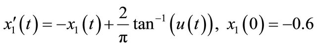
 (12)
(12)
It is required to minimize the following optimal criterion
 (13)
(13)
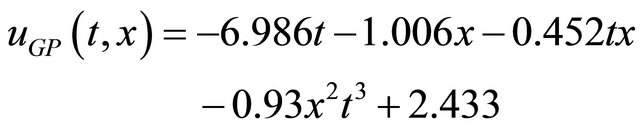
The MBFGP combined with numeric constant mutation is proposed to evolve the optimal control laws. The MBFGP algorithm is enforced to evolve three control laws uGP(t), uGP(x), and uGP(t, x). The terminal sets for the three controllers are: T = {t, one}, T = {x1, x2, x3, one}, and T = {x1, x2, x3, t, one} respectively, while the function set in all cases is F = {*, /, ^}. The MBFGP is also initiated to similar setting as in the previous problems. The following three control laws are evolved in generations 94, 74, and 88 respectively.

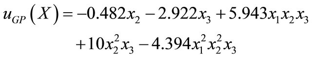
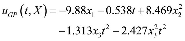 (14)
(14)
Figures 3 and 4 show the plots of the system states and the optimal control respectively for all GP solutions.
4. Conclusions
The standard GP algorithm is enhanced by creating a new tree structure. The crossover, the inverse shrink mutation, and the branch mutation operations are split into
Table 2. MBFGP and CVP method solutions.
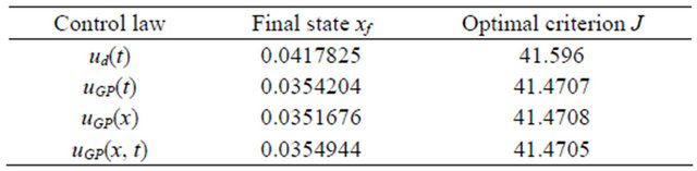
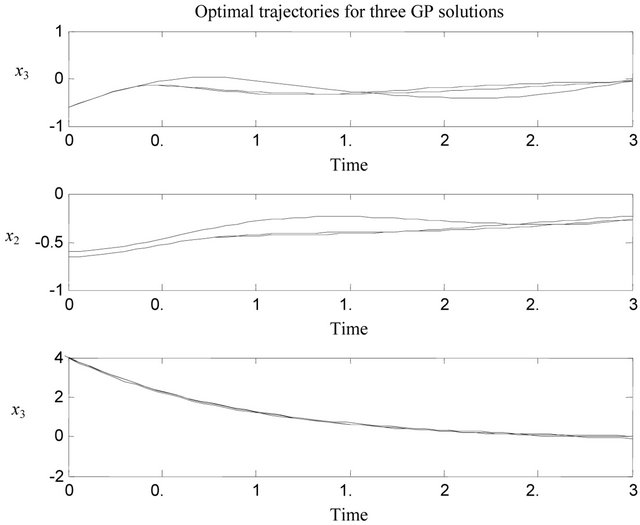
Figure 3. System states when GP solutions are applied.
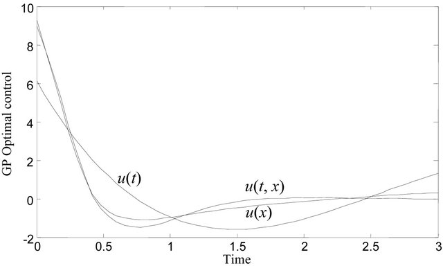
Figure 4. Optimal control u* for all GP solutions.
two operations (internal and external) with different probabilities.
Moreover, four new operations are added, the delete, contribution, merging and endowment operations, which are controlled by specific probabilities and special parameters. Therefore, a new algorithm named MBFGP is performed.
The MBFGP algorithm can be used efficiently to synthesize an optimal (or very near optimal) control law for linear as well as nonlinear systems. MBFGP algorithm deals with them all similarly without significant change. In addition, the MBFGP algorithm has the capability of determining beforehand the independent variables in the evolved optimal controller. The obtained results show that the MFBGP algorithm can evolve different controllers as many as the different terminal sets.
REFERENCES
- J. R. Koza, “Genetic Programming: On the Programming of Computers by Means of Natural Selection,” The MIT Press, Cambridge, 1992.
- D. J. Montna, “Strongly Typed Genetic Programming,” Evolutionary Computation, Vol. 3, No. 2, 1995, pp. 199- 230. doi:10.1162/evco.1995.3.2.199
- E. Hemberg, C. Gilligan, M. O’Neill and A. Brabazon, “A Grammatical Genetic Programming Approach to Modularity in Genetic Programming,” Proceedings of the Tenth European Conference on Genetic Programming, Valencia, 11-13 April 2007. doi:10.1007/978-3-540-71605-1_1
- I. G. Tsoulos and I. E. Lagaris, “Solving Differential Equations with Genetic Programming,” Genetic Programming and Evolvable Machines, Vol. 7, No. 1, 2006, pp. 33-54. doi:10.1007/s10710-006-7009-y
- C. Yuehui, Y. Ju, Y. Zhang and J. Dong, “Evolving Additive Tree Models for System Identification,” International Journal of Computational Cognition, Vol. 3, No. 2, 2005, pp. 19-26.
- J. Imae and J. Takahashi, “A Design Method for Nonlinear H∞ Control Systems via Hamilton-Jacobi-Isaacs Equations: A Genetic Programming Approach,” Proceedings of 38th conference on Decision & Control, Phoenix, 7-10 December 1999.
- J. Imae, et al., “Design of Nonlinear Control Systems by Means of Differential Genetic Programming,” 43rd IEEE Conference, Atlantis, 14-17 December 2004.
- M. Evett and T. Fernandez, “Numeric Mutation Improves the Discovery of Numeric Constants in Genetic Programming,” Proceeding of the Third Annual Genetic Programming Conference, Madison, 22-25 July 1998, pp. 66- 71.
- L. S. Lasdon, S. Mitter and A. Waren, “The Method of Conjugate Gradient for optimal Control Problems,” IEEE Transactions on Automatic Control, Vol. AC-12, 1967.
- A. M. Rami, “Optimization and Optimal Control, Lecture Notes,” University of Technology, Baghdad, 1995-2003.
- M. J. Mohamad, “A Proposed Genetic Programming Applied to Controller Design and System Identification,” Ph.D. Thesis, University of Technology, Baghdad, 2008.
- M. Noton, “Modern Control Engineering,” Pergamon Press Inc., Oxford, 1972.
Appendix—Contribution Operation Algorithm
- Let j = 1.
- Start a loop.
- Consider the current basis functions in the individual i and compute its standard fitness Sf(t).
- Store the original values of the numeric constant terminal nodes of the individual i and record their locations.
- Hide the basis function j that requires computing its contribution.
- Optimize the values of the numeric constant terminal nodes of the remaining basis function in the individual using the proposed numeric constant mutation or any available technique (use predetermined iterations).
- Compute the standard fitness  of the individual i when the basis function j has been hidden.
- If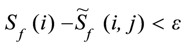 , then delete the basis function j from the considered individual, where Sf(t) is the standard fitness with the basis function j,
  is the standard fitness without basis function j, ε is the error reduction value (very small positive value).
- Else, return the basis function j in the individual i and return the original values of the numeric constant terminal nodes to their original locations in the individual i.
- j = j + 1.
- Go to “Start a loop” to choose another basis function.
- The above steps will be repeated, but this time it will be applied to a combination of two basis functions. All such possible combinations will be con.