Received 2 April 2015; accepted 2 June 2015; published 5 June 2015

ABSTRACT

Different aspects of mathematical finance benefit from the use Hermite polynomials, and this is particularly the case where risk drivers have a Gaussian distribution. They support quick analytical methods which are computationally less cumbersome than a full-fledged Monte Carlo framework, both for pricing and risk management purposes. In this paper, we review key properties of Hermite polynomials before moving on to a multinomial expansion formula for Hermite polynomials, which is proved using basic methods and corrects a formulation that appeared before in the financial literature. We then use it to give a trivial proof of the Mehler formula. Finally, we apply it to no arbitrage pricing in a multi-factor model and determine the empirical futures price law of any linear combination of the underlying factors.

Keywords:

Hermite Polynomials, Multi-Factor Model, Hilbert Space, Mehler Formula

1. Introduction

Hermite polynomials are widely used in finance, for various purposes including option pricing and risk man- agement. Madan and Milne [1] have built a framework applying functional analysis results to the particular case of Hermite polynomials and inferred pricing formulas for general payoffs expressed as linear combinations of Hermite polynomials. They applied their framework to the simple case of calls to determine the implicit basis prices in the market data and imply an empirical futures price law. More recently, a series of papers have de- veloped closed-form series expansions for various models: Tanaka, Yamada and Watanabe [2] developed ap- proximations of the prices of some interest derivatives; Schloegl [3] adapted this type of expansions to multi- period models. On the other hand, Buet-Golfouse and Owen [4] , Voropaev [5] , and Owen et al. [6] applied the Mehler formula and multivariate Hermite expansions to the allocation of risk measures in a portfolio of financial instruments.

The aim of this paper is to derive a theoretical framework that underlies many usages of Hermite polynomials in finance. In particular, the first main result of this paper is to have established a link between the probability distribution of the underlying factor and the empirical prices of Hermite functions. The second main result is a multinomial expansion theorem for Hermite polynomials (and its extensions). Both provide a solid foundation to derive the no-arbitrage price of a contingent claim stemming from a linear combination of factors.

The article is organised as follows: in the first section we state some basic facts about univariate and multi- variate Hermite polynomials; the second section is devoted to the justification of expansions on the basis of Hermite functions and demonstrates the link between implicit prices of Hermite polynomials and the probability distribution of the underyling assets under the forward probability measure; the third section states and proves a multinomial theorem for Hermite polynomials with extensions and examples provided in the fourth and fifth sections; the sixth and final sections are dedicated to the application of the multinomial theorem for Hermite polynomials to pricing under no-arbitrage. Finally, empirical applications of the described methodology can be found in [4] and [6] .

2. A Few Facts about Hermite Polynomials

Our objective is not to give a full account of the literature on Hermite polynomials but simply to recall some definitions and properties (see Abramovitz and Stegun [7] for more information). Let be the standard normal density and be the Hermite polynomial satisfying and for any,

. An alternative definition is via the exponential generating function

.

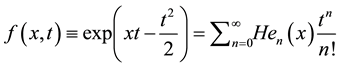The two most important properties are the recurrence relationship and the orthogonality property. The re- currence relationship states that,:

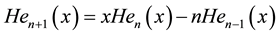(1)

and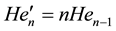, whilst the orthogonality property states that for all

(2)

Explicit and inverse explicit expressions are available for Hermite polynomials: for all and, the following identities hold:

(3)

N-multivariate Hermite polynomials are usually defined as the product of N univariate Hermite polynomials. Let us first clarify some notations used in the rest of the paper:, are vectors respectively in and, is the Euclidian scalar product in, while refers to the generalised factorial, i.e., so that for any, and is the order of n.

is defined as

(4)

The orthogonality property can readily be adapted to the multivariate case component by component:

(5)

Let us now consider the Hilbert space of functions that are square integrable with respect to the measure P defined by the density

(6)

An orthonormal basis for H is given by the polynomial functions (also sometimes called “Hermite

functions”):

Using standard arguments in functional analysis, an arbitrary claim in H may be expressed in the basis as

(7)

where the coefficients are obtained by the Hilbertian inner product

(8)

To summarise, we have built an orthonormal basis in which to decompose functions that are square-integrable against the standard N-dimensional Gaussian distribution

(9)

but have actually made no assumption on the distribution of the vector of factors. Indeed, this is the subject tackled by the following section.

3. Implied Prices and Probability Distributions

In this section, we demonstrate the link between two notions that are used separately in the literature: the implicit prices of Hermite polynomials (as in Madan and Milne (1994), where the payoff is expanded in Hermite polynomials) and the risk-neutral distribution of the vector of factors (see Yamada and Watanabe [2] and Schloegl [3] where it is the factors’ density that is expanded in Hermite polynomials and not the payoff as such).

We consider a financial market on a period with: where is the uni- verse, the chosen -algebra (assumed here to be the Borelian tribe) and the market’s probability mea- sure (a priori, it is not necessarily a risk neutral measure, as we can choose it to be the physical measure). We denote by the risk-free rate and the related zero-coupon with time horizon T. Note that we consider this simple framework to lay out the assumptions and theorems, but it could be adapted to a multi- period setting. In the definition below, we summarise the key aspects of a complete market (see Portait and Poncet [8] ).

Proposition 1. A self-financing strategy is admissible if its terminal value is a random variable whose second moment is well-defined (i.e., it is square-integrable), a contingent claim is attainable if there exists a self- financing strategy whose terminal value is equal to the contingent claim almost surely (in particular, it has to be square integrable), and the market is complete if all contingent claims are attainable. A system of prices V is an application from the set of contingent claims to and it is said to be viable if it is compatible with the no- arbitrage condition: in particular, it is a linear form.

From now on, we assume the market to be complete and to satisfy the no arbitrage condition and consider to be the risk-neutral measure (and to be absolutely continuous with respect to the Lebesgue measure).

If, then it is attainable and has a unique price (V is also unique) and further assum-

ing that, it can be expanded in the basis of Hermite polynomials. This results in the possibility

to express the contingent claim as a linear combination of the basis elements, namely the Hermite functions, which can be seen as simpler contingent claims. Using the linearity of the price functional V and Cauchy-Schwarz inequality (see Theorem 2.2 in Madan and Milne [1] ), this finally yields the market value of as

(10)

with the (implicit) market price of.

Theorem 1. Under the assumption that V is continuous there exists a unique such that for all,

(11)

Proof. We already know that V is a linear form on (which is a Hilbert space) and under the theorem’s assumption, it is also continuous. Hence, using the Riesz representation theorem (see Brezis [9] ), we

can infer the existence of a unique such that. □

We now turn to the probability density function and its (unique) Radon-Nikodym derivative with respect to the reference measure P defined as the N-variate standard Gaussian distribution in the previous section, that is:

(12)

so that, finally, we have

(13)

Definition 1. Under the same assumptions, is called the futures price law of with respect to the probability measure P.

The meaning of the futures price law can be derived as follows: rewriting as

(14)

it becomes clear that is the inner product in of the payoff and the empirical prices law (which makes sense if the latter is square integrable). We now give a theorem linking the futures price law, prices of the basis elements and Hermite expansions to translate this observation in rigorous terms.

Theorem 2. The following statements are equivalent:

i) There exists a sequence, such that and for any such that;

ii);

iii) There exists a sequence, such that and.

Remark 1. This result is a slightly different view of Madan and Milne’s Theorem 4.1 [1] because our set of assumptions is minimal and it was derived following the path of the Riesz representation formula. In particular Madan and Milne’s assumption that is uniformly bounded above and below implies that .

Proof. Clearly, ii) implies iii). To prove that iii) implies ii), we apply Lemma 5.1. in Ch. 5 of Brezis [9] : the

sequence is in, its components are orthogonal to each other and

(15)

so that

(16)

Then, noting, it comes that exists and

.

It now remains to prove that i) is equivalent to iii). iii) implies i) is a simple consequence of the inner product in a Hilbert space:

(17)

Starting from i), we have that so that we can build which verifies

for any contingent claim that is also in. Hence, must equal. □

This theorem thus shows that under mild conditions (i.e. that the probability is not too “different” from P) the futures price law can be expanded in the basis of Hermite functions and is such that its coefficients are the prices of the Hermite functions under the risk neutral measure. But so far, we have simply considered V from a theoretical perspective and since we want to prove the link between our results and Yamada and Watanabe’s expansions in terms of the density of the factors, we can express it directly as

(18)

where r is the risk-free rate.

Introducing the risk-neutral T-forward measure, the following holds:

(19)

where is the price of the zero-coupon of horizon T (see [8] for details). A first but important remark is

that if r is assumed to be bounded, then so that we can consider contingent claims

under either probability measure. As in Tanaka et al. [2] , the assumption is made that the probability distribution g of under the T-forward measure can be expressed as

(20)

A sufficient and necessary condition for g to be a valid density function is to have

・ .

・ and for all.

Schloegl [3] discusses ways to ensure that the second condition is met in practice when the summation is taken over a finite number of Hermite functions. Now, using the pricing formula under the T-forward measure leads to:

(21)

When the various assumptions of the theorems above are verified, it comes

(22)

whence the following theorem linking the futures price law and the T-forward probability density function of the factors holds.

Theorem 3. The implied prices of Hermite functions and the coefficients of the the T-forward probability density function satisfy the fundamental equality

(23)

for all.

A direct application of this theorem is the determination of price elements from the moments of the distribution g and vice-versa. For the sake of clarity we consider the case in the rest of the section, but the results can easily be extended to the multivariate case.

Lemma 1. Let denote the moment of the distribution g:. Then

(24)

(25)

Proof. It suffices to use the explicit and inverse explicit formulas and perform some simple algebra to obtain both results. □

Since in the financial framework considered so far, all moments of the distribution g can be

implied from the prices of the orthonormal basis. Now that the foundations of the framework have been laid, we can move to another result, namely the Hermite multinomial theorem.

4. Factor Models and the Hermite Multinomial Theorem

Considering several factors at the same time and linear combinations of those is at the core of many financial models: Fama and French’s three-factor model for asset returns, Brennan and Schwarz’ two-factor model, Lang- estieg’s multi-factor model for interest rates or the multi-factor Merton-Vasicek model for example. Supposing that we have a financial instrument depending on a linear combination of the original factors, we would like to expand this instrument in the basis of Hermite functions: this has implications in terms of pricing and risk management as the factors can represent some macroeconomic variables that one might wish to stress. This section therefore states and proves a multinomial theorem for Hermite polynomials and corrects a previous expansion given by Voropaev in [5] .

Let us start by considering the example of a two-factor model, i.e.. Noting that and for any and, it simply comes

. (26)

Let us now compute separately:

(27)

Hence, in the case where, the following identity holds:

. (28)

The condition is absolutely key in the equality and is called the “factor loading condition” in credit risk modelling. It can actually be seen as a normalisation constraint: if and are independent and normalised (i.e. have mean 0 and variance 1), then will have mean 0 and variance 1 if and only if. We can now proceed to a general version of the theorem. This result did not have a general statement and proof widely available, but given its simplicity, it might have been derived in a different context.

Theorem 4. Let and. Then for all s with such that,

. (29)

Remark 2. The theorem can be restated in a more condensed form and in terms of Hermite functions as

. (30)

We offer two proofs of the result, one based on the repeated application of the recursion property (see the Appendix) and the other on the generating function of Hermite polynomials to show how powerful and different these two tools are for analysing relationships involving Hermite polynomials. They offer different insights in the manipulation of Hermite polynomials and are a good exercise for the reader.

Let us now move to a demonstration based on the exponential generating function.

Proof. We have that

(31)

Hence, comparing the first and the last lines of this equation we must have

(32)

which yields the result. □

To show how powerful this simple tool is, we provide some direct extensions and examples in the next two sections.

5. Two Extensions of the Multinomial Theorem

It is possible to easily extend this result to multivariate Hermite polynomials and to weights which do not re- spect the factor loading condition.

Looking first at the case of multivariate Hermite polynomials, the idea is to consider a linear combination of

multivariate factors so that is yet another vector.

Theorem 5. Let, , such that and. Then the following equality holds:

with the vector of the coordinates of the factors.

Proof. It suffices to apply the multinomial theorem for Hermite polynomials to each of the univariate Hermite

polynomials. □

Another extension, perhaps more important for practitioners, is to consider the case where the factor loading condition is not verified. For the sake of simplicity, let us go back to the univariate case and suppose that (but still). We can state the general multinomial theorem for Hermite polynomials as follows:

Theorem 6. Under the assumption that (i.e.), the following identity is checked:

. (33)

In the proof, we make use of the following lemma from Schloegl (2013) [3] :

Lemma 2. Let. Then

. (34)

Proof. (Of the theorem) We can rewrite as

. (35)

We derive the following equality from the intermediary lemma:

(36)

□

Remark 3. In the same vein, it is also possible to infer a similar but even more general result for

(37)

where and and even extend it to the multivariate case; we leave the computational details to the interested reader.

6. Revisiting the Orthogonality Property and the Mehler Formula

Let us revisit the orthogonality property, but this time in presence of correlation. Our aim is to compute, where X and Y are two standard Gaussian random variables with correlation coefficient. To do so we prove the following theorem.

Theorem 7. For any, the following identity is true:

(38)

with the Kronecker symbol and the bivariate Gaussian probability distribution function.

Proof. Another way of expressing this double integral is to write it as

. (39)

Using the binomial formula, which is a particular case of the multinomial formula that we have proved, we have

. (40)

Thus,

(41)

The “correlated orthogonality” property has been proved. □

Based on this simple observation, a simple and elegant proof of the Mehler formula can be given:

Corollary 1. (Mehler formula) The bivariate normal probability density function satisfies the following equality (for and):

. (42)

Proof. It suffices to expand in the Hermite polynomial basis:

(43)

and use the correlated orthogonality property. □

The Mehler formula is of special importance since it can be used as a foundation in credit-risk modelling, as in Voropaev [5] , to compute the expected value of a portfolio V of K financial instruments, , conditional on the value of a factor, say Y. Suppose that each is a function (verifying all necessary inte- grability conditions) of a random variable which depends linearly on a systemic factor Y and an idio- syncratic (i.e. instrument-specific) factor (’s are assumed to be mutually independent and to follow standard Gaussian distributions):

. (44)

Thus,. Focusing on, we can write the following equations:

(45)

where we have defined, which does not depend on the decomposition in

terms of Y and. This is extremely useful as it can be used for assessing the impact of Y on the whole port- folio (for instance by computing the value-at-risk of the conditional expected loss, and so on).

7. The Multinomial Factorisation Theorem and Arbitrage

Going back to our framework where the market has no arbitrage and is complete, we wish to determine the relationship between the implied prices of the basis and those of a linear combination of the underlying factors. To make things clearer suppose that we are looking at a payoff whose underlying factor is a linear combination of N factors (as previously, we note) with a vector of factor loadings whose norm is 1: with. Then:

(46)

which can be restated in terms of Hermite functions as where.

On the one hand, we have the basis of Hermite functions to expand the payoff as a function of:

(47)

where.

On the other hand, we can express the payoff of as a multivariate function of by writing that. Applying a multivariate expansion this time, we obtain that

(48)

where

(49)

Since, using the valuation formula, by no arbitrage, we would necessarily have

so that

(50)

where is the potential implied price of for all k and is the known implied price of

.

Thanks to the multinomial factorisation, we have that

. (51)

By identifying terms in this multivariate polynomial function, we obtain

. (52)

Turning to the prices, we see that

(53)

On the other hand, we have that. Bringing both equations together, we can write the following equality:

(54)

and infer the theorem:

Theorem 8. Since the function is a generic payoff, by analysing the series coefficient by coefficient, we finally obtain that

(55)

Proof. We have shown that was a valid choice for. Let us show that it is the only one by applying no-arbitrage pricing arguments.

Indeed, suppose that there exists such that (for clarity’s sake,). Let us then choose, which is a valid payoff, so that we have. A portfolio can then be built by buying the

duplicated payoff at price, i.e., and shorting it at price.

Since the payoffs and are equal, we have built a portfolio that displays an arbitrage. □

To summarise, we have shown that it was possible to express explicitly the coefficients and the prices as functions of the coefficients and the prices. The strength of this theorem is to make explicit the no arbitrage relationship between the empirical prices of the Hermite polynomials and the empirical price of a linear combination of the factors, which leads to the formulation of the following result:

Theorem 9. We have determined the futures price law density of denoted by as

. (56)

8. Concluding Remarks

This paper proposes a simple way of expanding the Hermite polynomial of a linear combination of factors into simpler elements. This method allows us to prove the celebrated Mehler formula in a very simple way, but also enables us to derive the empirical prices of functions of linear combination of factors in a market with no arbi- trage and facilitates credit risk modelling. Practical illustrations of the theoretical framework developed in this paper can be found in [2] - [6] . We have built on the theory developed by Madan and Milne and highlighted the relationship that existed between their results and other recent results obtained in the field of pricing. Using a multinomial theorem for Hermite polynomials, we have shown how to tackle expressions including more than one factor.

The main assumption made throughout the paper is the existence of a payoff’s or probability density func- tion’s expansion in the basis of Hermite polynomials. Although this is quite restrictive (it implies the existence of all moments in the latter case for instance), it does allow for significant deviations from the benchmark case of standard Gaussian distributions. The computational approach at hand indeed permits to only consider a series of simple computations rather than a difficult and time consuming one. It offers a practical analytical alternative to full-fledged Monte Carlo simulations.

Acknowledgements

The author would like to thank Anthony Owen and James Bryers for initiating this work on the use of Hermite polynomials in finance and their insightful remarks. Thanks also go to Li Shanqiu and to two anonymous referees for their helpful comments.

References

Appendix

In this appendix we give an alternative proof of the multivariate theorem for Hermite polynomials

Proof. The cases and, for all N, are obvious since and. Let us now suppose that the property holds for all k such that.

Using the recurrence formula

(57)

we can write that

(58)

We can split the above expressions into the three pieces:

(59)

(60)

(61)

Our aim is to demonstrate where

(62)

We start by proving and then move on to showing that.

(63)

Turning to, it now boils down to making the change of variables to obtain the equality

.

Similarly, in, using the change of variables, we obtain

(64)

Finally, the result has been proved. □

References

- Madan, D. and Milne, F. (1994) Contingent Claims Valued and Hedged by Pricing and Investing in a Basis. Mathematical Finance, 4, 223-245. http://dx.doi.org/10.1111/j.1467-9965.1994.tb00093.x
- Tanaka, K., Yamada, T. and Watanabe, T. (2010) Applications of Gram-Charlier Expansion and Bond Moments for Pricing of Interest Rates and Credit Risk. Quantitative Finance, 10, 645-662. http://dx.doi.org/10.1080/14697680903193371
- Schloegl, E. (2013) Option Pricing Where the Underlying Assets Follow a Gram/Charlier Density of Arbitrary Order. Journal of Economic Dynamics and Control, 37, 611-632. http://dx.doi.org/10.1016/j.jedc.2012.10.001
- Buet-Golfouse, F. and Owen, A. (2015) The Application of Hermite Polynomials to Risk Allocation. Barclays Quantitative Credit, Working Paper.
- Voropaev, M. (2011) An Analytical Framework for Credit Portfolio Risk Measures. Risk, November, 72-78.
- Owen, A., Bryers, J. and Buet-Golfouse, F. (2015) Hermite Polynomial Approximations in Credit Risk Modelling with PD-LGD Correlation. Journal of Credit Risk, Accepted Paper.
- Abramowitz, M. and Stegun, I. (1964) Handbook of Mathematical Functions. Dover Publications, New York.
- Portait, R. and Poncet, P. (2009) Finance de marche. 2nd Edition, Dalloz, Paris.
- Brezis, H. (2011) Functional Analysis, Sobolev Spaces and Partial Differential Equations. Springer, New York.