Applied Mathematics
Vol.4 No.1A(2013), Article ID:27506,6 pages DOI:10.4236/am.2013.41A039
Finite Element Solution of a Stream Function-Vorticity System and Its Application to the Navier Stokes Equations
1Equipe Modélisation Mathématique et Simulation, Faculté des Sciences Université Ibn Zohr, Agadir, Maroc
2Institut Jean Rond d’Alembert/CNRS, UPMC Université, Paris, France
Email: f.ghadi@uiz.ac.ma, m.wakrim@uiz.ac.ma, ruas@lmm.jussieu.fr
Received October 6, 2012; revised November 28, 2012; accepted December 5, 2012
Keywords: Characteristics Method; Navier-Stokes; Stream Function; Vorticity
ABSTRACT
The finite element solution of a generalized Stokes system in terms of the flow variables stream function and vorticity is studied. This system results from a time discretization of the time-dependent Stokes system in stream function-vorticity formulation, or yet by the application of the characteristics method to solve the Navier-Stokes equations in the same representation. Numerical results presented for both cases illustrate the good behaviour of the adopted approach.
1. Introduction
Expressing the incompressible Navier-Stokes equations in terms of variables other than velocity and pressure becomes a good alternative for solving them numerically, provided one is able, not only to uncouple the new flow variables, but also to derive reliable discrete counterparts. In this respect the classical stream function and vorticity formulation of these equations in two-dimension space is a very good example. After having studied it in the stationary case (cf. [1]), in this paper we generalize our results [1] to the time-dependent problem.
In terms of numerical analysis this paper primarily deals with a mixed method to solve the two-dimensional generalized Stokes problem in terms of the stream function and the vorticity. Such problem results for instance from the time discretization of the time-dependent Stokes system. The difficulty arising from the lack of boundary conditions for the vorticity is overcome by means of a suitable technique for uncoupling both variables following the mains lines of the well-known Glowinski-Pironneau method [2]. Then we discretize in space the resulting uncoupled system by means of continuous Lagrange finite elements.
In computational terms we apply the above technique to the Navier-Stokes equations. This is achieved by first performing the semi-discretization in time of these equations by a classical characteristics method. Then we apply the same numerical ingredients as for the generalized Stokes system. We illustrate the good performance of our approach by means of numerical results, obtained for some benchmarks problems such as cavity lid driven flow.
2. The Time-Dependent Stokes System as a Model Problem
Given a field of volumetric forces f with  for any time t, and denoting by ν the kinematic viscosity of the fluid occupying a bounded simply connected domain Ω of R2 with boundary Γ assumed to be Lipschitz continuous, we wish to find the stream function
  and the vorticity ω such that
 (1)
(1)
where  and
and  are functions determined from the given velocity on
 ![]() for every
for every , together with an appropriate initial condition at time
 .
.
The Euler type implicit discretization in time of system (1) with time step  gives
gives
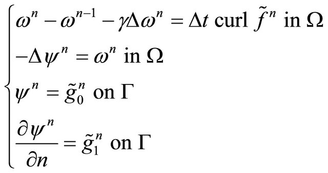 (2)
(2)
where  with
with  given, and
  for any function
 .
.
Assume that ![]() is known. Then problem (2) becomes a generalized Stokes problem.
is known. Then problem (2) becomes a generalized Stokes problem.
If we omit the index![]() , the problem is written
, the problem is written
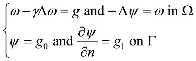 (3)
(3)
where  and
and ,
,  and
and  are given.
3. Variational and Uncoupling Techniques
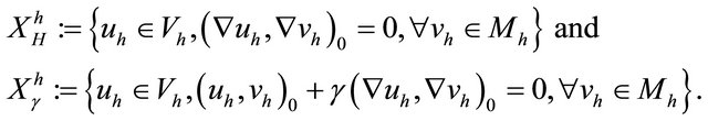
Like in [1], a suitable variational formulation of system (3) is provided by using the space
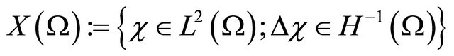 . In order to uncouple the resulting system we work with the spaces
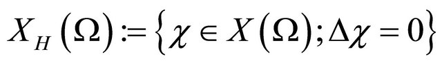
and 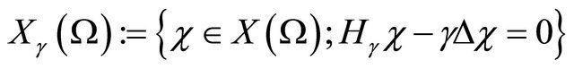 .
.
Now using standard arguments, we may uniquely write every function  as a sum of the form
 , where
  is uniquely defined by
  and
and . Then letting
 , where
  and
and and recalling that
  and
and
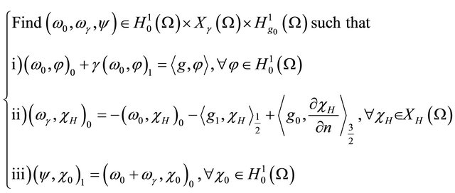
 (cf. [1]), the uncoupled formulation associated with system (3) is: (see Equation (4))
where  and
and denotes the duality product between
  and
and  with
with . Problem (4) has a unique solution
 , which is such that the field
  is the unique solution of system (3).
4. Discretized Problem
The type of finite element approximation of problem (4) was first introduced in [3]. In this work we develop it in detail by referring the reader to that work for the numerical analysis of the method. Assuming that  is a polygonal domain and letting
  be a quasiuniform family of triangulations of
  with mesh step size
 , we introduce the finite element spaces defined by:
Here  denotes the space of polynomials of degree less than or equal to
 , defined in an element
  and
and  is the numbered set of all the nodes used to define the degrees of freedom of
  that lie on
![]() .
.
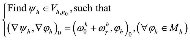
Finally, we define
Then the discrete versions of problems (4-i), (4-ii) and (4-iii) are defined as follows: (see Equation (5)).
We note that the determination of  and
and  requires the computation of a basis of
  and another one of
 .
.
The following algorithm describes how to compute these bases and how to determine  and
and .
.
 (4)
(4)
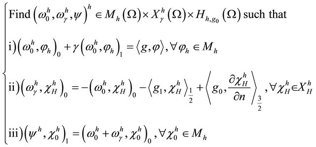 (5)
(5)
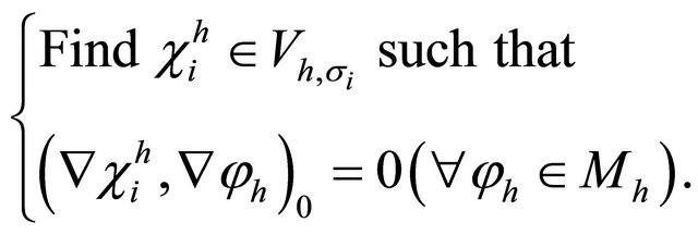
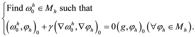
Algorithm
Step 1
For  compute
 :
:
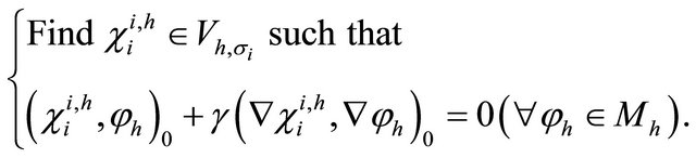
Step 2
For  compute
 :
:
Step 3
Step 4
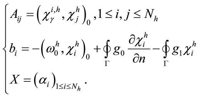
Compute 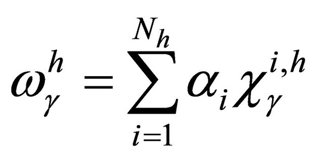 by solving the linear system
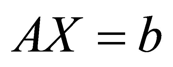 , with
Step 5
5. Numerical Experiments
In order to illustrate the performance of our approach, we present some numerical results obtained in the framework of a problem with known solution, solved with the equal order method for .
.
We consider the stationary Stokes problem in 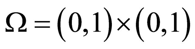 , whose exact solution is given by
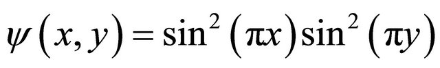
and
 .
.
In this example de mesh is 30 × 30, and we run a sufficient number of time steps to reach a stationary solution, with reasonable accuracy.
In Figure 1 we display the contours of the exact and approximate vorticity for , respectively on the left and on the right. In Figure 2 we display the contours of the exact and approximate streamlines for
 , respectively on the left and on the right. In Figure 3 we display the exact and approximate vorticity along the first diagonal. In Figure 4 we display the exact and approximate stream function along the first diagonal.
6. Extention to the Navier-Stokes Equations
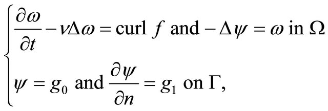
Let us first recall the Navier-Stokes equations expressed in the stream function and vorticity formulation.
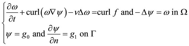 (6)
(6)
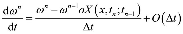
We use the method of characteristics of first order for the time-discretization of the vorticity particle derivative, namely
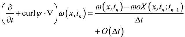 (7)
(7)
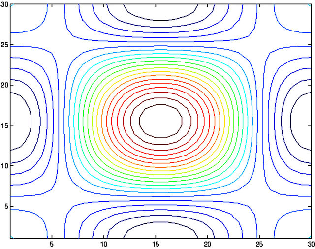
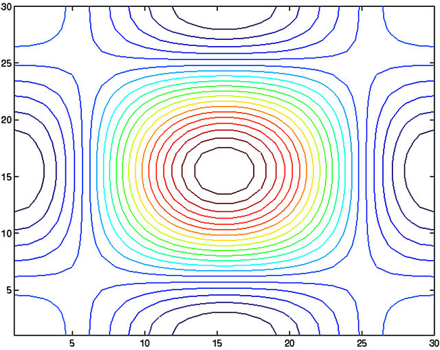
Figure 1. Exact (left) and approximate (right) vorticity contours.
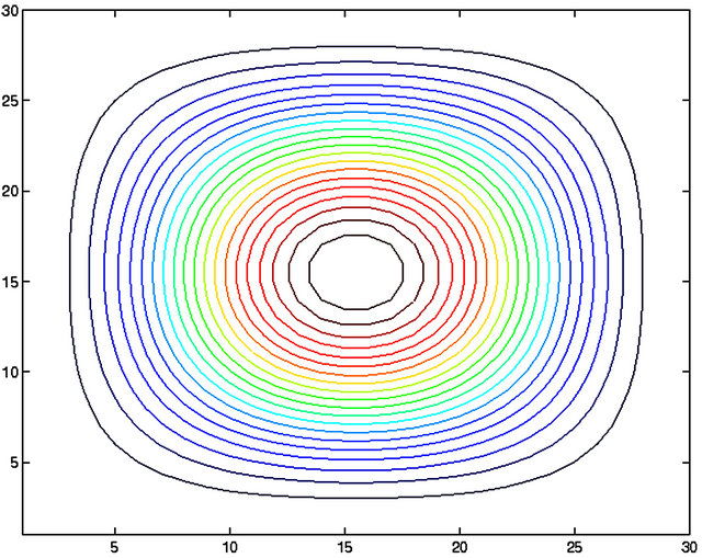
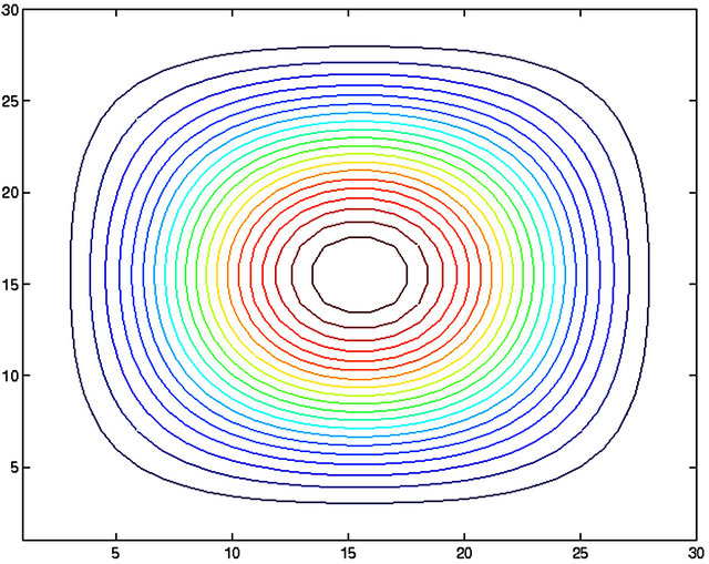
Figure 2. Exact (left) an approximate (right) streamline.
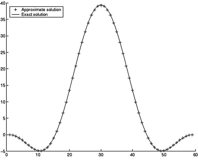
Figure 3. Exact an approximate vorticity along the first diagonal.
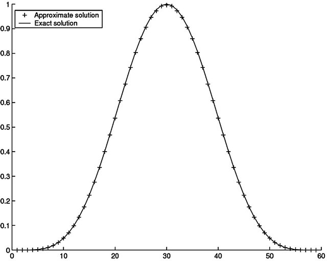
Figure 4. Exact an approximate stream function along the first diagonal.
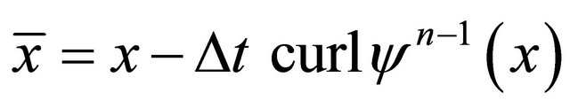
 is the solution of the problem:
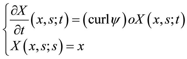 (8)
(8)
We obtain:
 (9)
(9)
from which we derive the scheme:
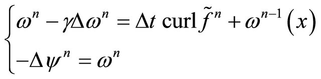 (10)
(10)
where
System (10) is nothing but a generalized Stokes problem problem of the type (3). Hence we can use the above described algorithm to solve it. The main difficulty is the computation of![]() .
.
7. Numerical Tests
In order to validate our approach, we present the driven cavity flow results.
In Figure 5 we display the streamlines and vorticity contours for . In Figure 6 we display the comparison along the first diagonal between the vorticity (respectively the stream function) obtained with the characteristics method and the one obtained with the linearization method employed in [4]. In Figure 7 we display the streamlines and vorticity contours for Re = 100.
The numerical results presented in this Section not only confirms the adequacy and economy of our approach to solve the incompressible Navier-Stokes in two-dimension space, but also illustrates that it can be
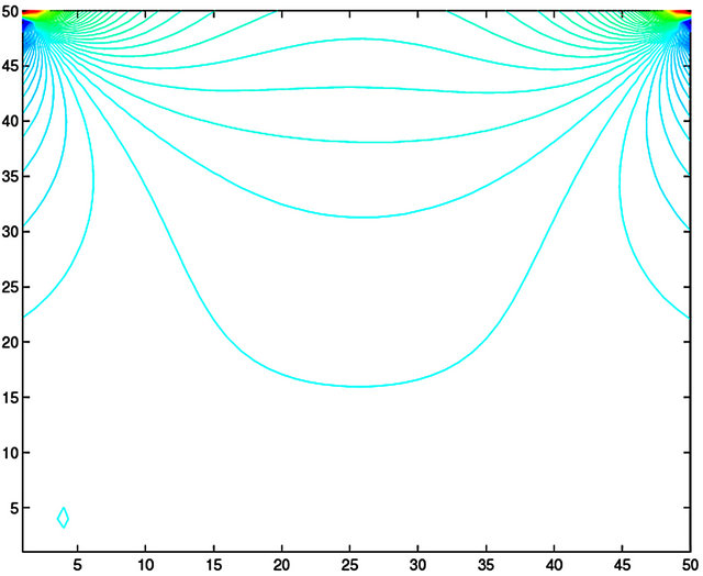
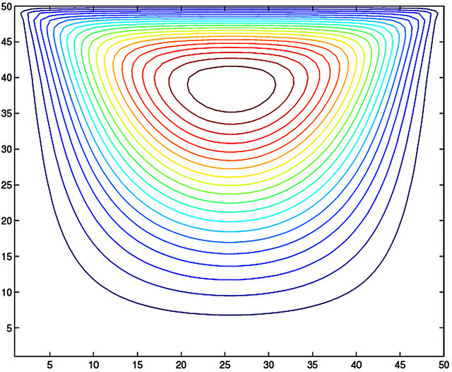
Figure 5. Re = 100. Vorticity computed with characteristic method, stream function computed with characteristic method.
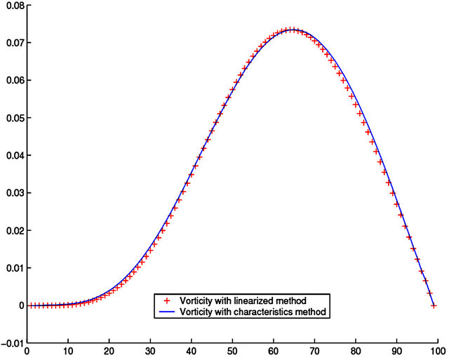
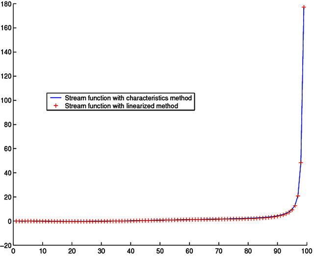
Figure 6. Re = 10. Comparison of the two solutions along the first diagonal.
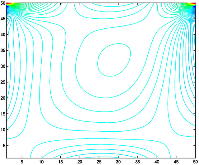
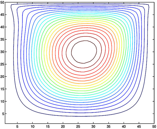
Figure 7. Re = 100. Vorticity computed with characteristics method, streamline computed with characteristics method.
suitably combined with the characteristics method. However the main difficulty of such combination is the choice of the time step . Unfortunately when the Reynolds number increases this issue becomes critical. In this case it is advisable to use moving meshes or yet a higher order characteristics method, in order to improve the quality of the numerical results.
REFERENCES
- F. A. Ghadi, V. Ruas and M. Wakrim, “A Mixed Finite Element to Solve the Stokes Problem in the Stream Function and Vorticity Formulation,” Hiroshima Mathematical Journal, Vol. 28, No. 3, 1998, pp. 381-398.
- R. Glowinski and O. Pironneau, “Numerical Methods for the First Bi-Harmonic Equation and for the Two-Dimensional Stokes Problem,” SIAM Review, Vol. 21, No. 2, 1979, pp. 167-212. doi:10.1137/1021028
- F. A. Ghadi, V. Ruas and M. Wakrim, “A Mixed Method to Solve the Evolutionary Stokes Problem in the Stream Function and Vorticity Formulation,” Proceedings of LUXFEM, Luxemburg, 13-14 November 2003.
- F. A. Ghadi, V. Ruas and M. Wakrim, “Numerical Solution to the Time—Dependent Incompressible NavierStokes Equations by Piecewise Linear Finite Elements,” Journal of Computational and Applied Mathematics, Vol. 215, No. 2, 2008, pp. 429-437. doi:10.1016/j.cam.2006.03.047