Applied Mathematics
Vol.5 No.16(2014), Article
ID:49480,12
pages
DOI:10.4236/am.2014.516245
Robust Optimization for Gate Sizing Considering Non-Gaussian Local Variations
Jin Sun, Janet M. Roveda
Department of Electrical and Computer Engineering, The University of Arizona, Tucson, USA
Email: sunj@email.arizona.edu, wml@ece.arizona.edu
Copyright © 2014 by authors and Scientific Research Publishing Inc.
This work is licensed under the Creative Commons Attribution International License (CC BY).
http://creativecommons.org/licenses/by/4.0/


Received 1 July 2014; revised 2 August 2014; accepted 11 August 2014
ABSTRACT
This paper employs a new second-order cone (SOC) model as the uncertainty set to capture non-Gaussian local variations. Then using robust gate sizing as an example, we describe the detailed procedures of robust design with a budget of uncertainty. For a pre-selected probability level of yield protection, this robust method translates uncertainty budgeting problems into regular robust optimization problems. More importantly, under the assumption of non-Gaussian distributions, we show that within-die variations will lead to varying sizes of uncertainty sets at different nominal values. By using this new model of uncertainty estimation, the robust gate sizing problem can be formulated as a Geometric Program (GP) and therefore efficiently solved.
Keywords:Robust Gate Sizing, Second Order Cone, Geometric Programming, Budget of Uncertainty, Parameter Variations

1. Introduction
Due to the decreasing feature sizes, the advanced sub-wavelength semiconductor fabrication techniques fail to control precisely dopant diffusion [1] [2] and are unsuccessful in printing geometric features accurately [3] . Consequently, a significant amount of process variations are introduced into the integrated circuits. These variations have caused substantial changes in the device and interconnect electrical parameters. The parametric yield of manufacture process and performance are thus in jeopardy. This is the main reason why process variations are the key topics of recent research studies.
Most research publications [1] -[3] classify process variations into inter-die or global and intra-die or local two components. Here, the global variations include variations between different chips, either in the same wafer or different wafers. Local variations include variations existing in different devices or interconnect within the same chip. Global variations are in general modeled as Gaussian distributed random variables. Local variations, on the other hand, are not easy to capture. One reason is that local variations, also random in nature, exhibit strong spatial correlations. To illustrate, two devices or interconnects are strongly correlated if they are spatially close to each other. If they are far apart, the correlations may be neglected. In addition, [4] and [5] have pointed out that it is not accurate to use Gaussian distribution to model local variations. In particular, [4] suggested a new statistical model, the Matern model, to capture the local variations based on the measurement data for 90 nm chips. The contributions of this paper can be summarized as follows. First, we propose a new Second-Order Cone (SOC) uncertainty model for characterizing parameter variations. This new SOC model extracts the quadratic and even higher order spatial variations with regard to correlations. Given certain probability for performance, we show how to translate budget uncertainty problems to yield-guaranteed robust optimization problems. By employing the SOC estimation model under yield-guaranteed timing constraints, we can translate the robust gate sizing problem into a standard GP formulation and conduct a budget of uncertainty between timing yield and gate size variations. Finally, we thoroughly verify the accuracy of our models against Gaussian distribution based models with a number of circuits. The rest of the paper is organized as follows. Section 2 describes the concepts of budget of uncertainty, non-Gaussian distributed variations and their impact on defining uncertainty set for variation estimation. Section 3 introduces the Second-Order Cone (SOC) estimation model for characterizing parameter uncertainties. Section 4 develops the proposed robust optimization technique by using the SOC uncertainty model and the notion of uncertainty budgeting. Section 5 demonstrates experimental results, and finally Section 6 concludes this paper.
2. From Uncertainty Budgeting to Robust Gate Sizing
Most research works on timing analysis and gate sizing use a posynomial function to model gate delay for individual components [6] -[10] . In [8] the authors proposed a class of generalized posynomial models to approximate gate delays. The timing constraints can be represented in the following form:
 (1.1)
(1.1)
where the j-th constraint function  represents the path delay at gate
 , which is in posynomial form.
If the multiplicative coefficients ’s are allowed to be any real number, then
  is called a signomial. As there are no restrictions on the sign of coefficients
 ’s, signomials are expected to estimate delay functions more accurately. In this work, we employ the signomial model for gate delay approximation. We use an automated procedure of posynomial/signomial fitting to determine the best-fit coefficients, exponents and the number of terms in the signomial delay function. The fitting procedure starts with a single monomial term for delay approximation, and gradually increase the number of monomial terms in the signomial function until the fitting error is less than a pre-determined threshold value.
Design optimization affected by process introduced variations has been a focus of recent research efforts [11] -[14] . How to formulate the design optimization depends on the models of variations. Indeed, it has also been pointed by [15] that “solutions to optimization problems can exhibit remarkable sensitivity to perturbations in the parameter”. Process variations are generally modeled as random variables. A nature way is to formulate design optimization affected by parameter uncertainty as a stochastic optimization problem. In this section we will use gate sizing, a typical circuit design problem, as an example to explain how to employing the notion of uncertainty budgeting to translate a in general NP-hard stochastic problem [16] into a tractable robust optimization problem.
Due to process variations, the components of vector , i.e. the gate sizes, have been assigned random variations around their nominal values. In this sense gate sizes are no longer deterministic quantities but random variables. As a consequence the gate delay becomes variational as well. Let
  represent the variations in gate sizes, the objective function
  and constraint function
  in (1.1) will be replaced by
  and
and  respectively. Therefore, the gate sizing problem under parameter uncertainties becomes the following stochastic optimization formation:
 (1.2)
(1.2)
As shown in (1.2), stochastic optimization tries to find the optimal nominal design parameters such that under the impact of parameter variations around these nominal values, the objective function is optimized in an average sense (i.e. the mean value), and constraints are satisfied with a probabilistic guarantee .
.
The most simplistic formation of uncertainty set is to use interval information and model a parameter under variation as a symmetric and bounded random variable  that takes values in
 . The halflength
  measures the precision of the estimate. Associated with the uncertain data
 , we define the random variable
  which obeys an unknown but symmetric distribution, and takes values in
 .
.
All resulting ’s form an uncertainty set:
 (1.3)
(1.3)
The main limitation of robust optimization is the lack of probabilistic description of parameter uncertainty and the conservativeness of optimization results due to the assumption of a complete guarantee of full yield. In this case, we might ask for probabilistic guarantees for the robust solution that can be computed a priori, i.e. as a function of the structure and size of the uncertainty set. This provides a notion of a budget of uncertainty, which allows the designer a level of flexibility in choosing the tradeoff between robustness and performance, and also allows the ability to choose the corresponding level of probabilistic protection. To be specific, the robust optimization with uncertainty budgeting can be formulated as:
 (1.4)
(1.4)
where stands for the uncertainty set, of which the size can be computed a priori given a pre-selected . Note that uncertainty set
  is usually modeled as a function of both nominal design parameters and probabilistic guarantee. Still use the example of interval uncertainty set (1.3) to interpret, we define a parameter as a budget of uncertainty for timing constraint:
 (1.5)
(1.5)
The parameter![]() , which belongs to
, which belongs to , is interpreted as the maximum number of parameters that can deviate from their nominal values. If
 , all
, all ’s are forced to 0, and there is no protection against uncertainty. If
 , the timing constraint is completely protected against uncertainty, which yields a very conservative solution. If
 , the designer makes a trade-off between the protection level of the constraint and the conservativeness of the solution. In later part, we show that by employing the concept of second order cone, there exists a convenient and efficient uncertainty set that provides such flexibility at different level of yield protection.
3. Parameter Variations and Uncertainties Characterization
The two main problems in budgeting uncertainty in robust optimization are to set up an appropriate uncertainty set for parameter uncertainty and establish the dependency of probabilistic guarantee on the structure and size of uncertainty set. This section first discusses estimation models for characterize parameter variability. We start with introducing the previously used UE method and its disadvantages. A new USOC method will then be proposed to overcome the limitations of UE method.
Ellipsoidal uncertainty set (UE) [11] [17] [18] is widely used to model parameter uncertainty, by using the maximal inscribed ellipsoid inside the variation region. For any vector  with random perturbation around its nominal value
 , the parameter variability can be estimated by an uncertainty ellipsoid in
 , which has the form [19] :
 (1.6)
(1.6)
where  represents the covariance matrix. The nominal vector
  is the center point of the uncertainty ellipsoid. An alternative representation of an uncertainty ellipsoid is:
 (1.7)
(1.7)
The vector ![]() is introduced to characterize the movement of
is introduced to characterize the movement of  around
 , and
, and  is the 2-norm of vector
![]() . The parameter variations are considered to be bounded within the ellipsoid region. Covariance matrix
. The parameter variations are considered to be bounded within the ellipsoid region. Covariance matrix  determines how far the uncertainty ellipsoid extends in every direction from
 . The lengths of radiuses
  and
and , and their directions are given by the eigenvalues of matrix
 .
.
In this work we propose a novel uncertainty set to model parameter uncertainties by employing the concept of a second order cone (SOC). Mathematically, a unit second order cone of dimension  is defined as [20] :
 (1.8)
(1.8)
where  is a vector of dimension
 . For the random vector
  of gate sizes, by introducing an auxiliary variable
 , the variation vector
  can be represented by a second order cone, which is defined as a set:
 (1.9)
(1.9)
where  is the 2-norm of variation vector
 . A general-form second-order cone can be extended from the unit case in (1.9):
 (1.10)
where problem parameters are ,
,  ,
,  and
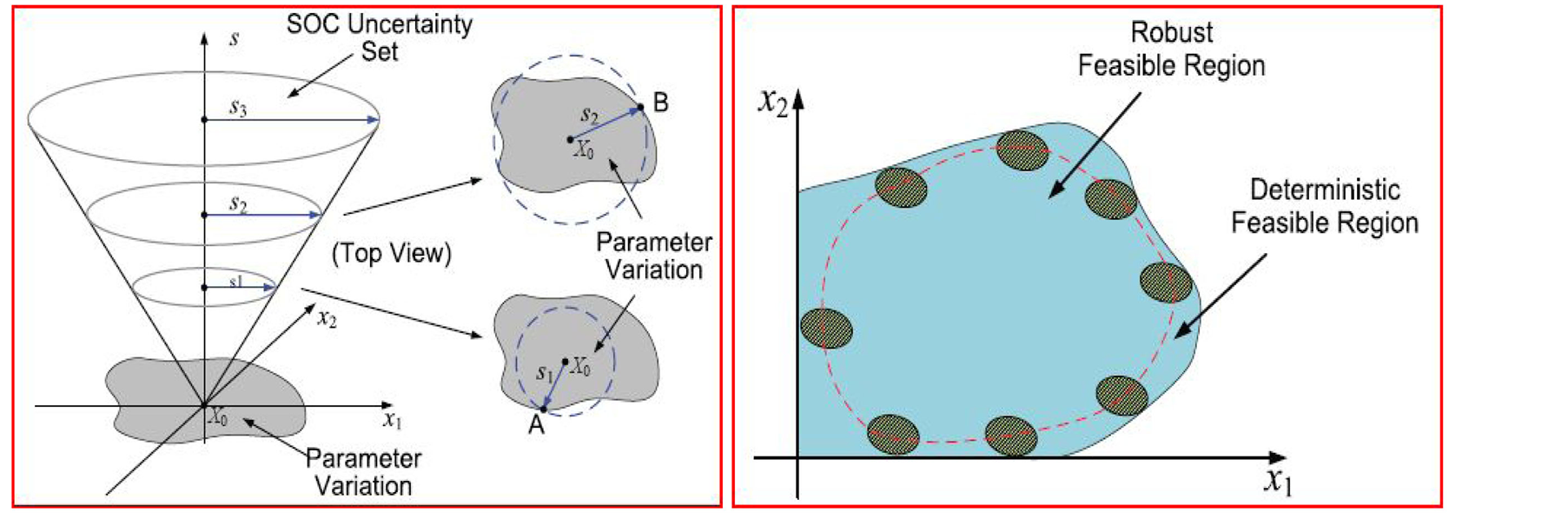
and . For illustrative purpose, in what follows we use the simple case of unit SOC to explain the advantageous of SOC uncertainty set over ellipsoidal uncertainty set. Referring to the example shown in Figure 1(a), a 3-dimensional (3D) cone has continuously changing radiuses to their 2D slices. The intersections of the 3D cone and feasible region thus provide the corner case distances to the nominal case. For example in Figure 1(a), the cone-feasible region intersection captures one corner case (Point A) with radius
![]() . If we push the cone through the feasible region continuously, more corner cases with different distance to the nominal point will be captured. As an example, a new corner point B is identified with a different radius
. If we push the cone through the feasible region continuously, more corner cases with different distance to the nominal point will be captured. As an example, a new corner point B is identified with a different radius . The elastic radius
 ![]() in fact restricts how far the parameter variations can perturb from their nominal values.
in fact restricts how far the parameter variations can perturb from their nominal values.
Having explained the formation of SOC uncertainty set, a nature question is how to determine an explicit form of  in terms of nominal design parameters. We use a fitting technique to find out the relationship between
  and nominal gate sizes by sampling gate size variations from their distribution information. As introduced before, local variations are difficult to capture, especially in the presence of strong spatial correlation. Following [4] [21] [22] the die can be considered as consisting of a grid of
  locations. A location on the chip will be denoted by
  where
where ![]() is the horizontal coordinate and
is the horizontal coordinate and ![]() is the vertical coordinate. Each grid field will be considered as a random variable with mean
is the vertical coordinate. Each grid field will be considered as a random variable with mean , where
  does not depend on the location
  but is dictated by the inter-die variations and varies from chip to chip. The parameter variations at any two locations
  and
and  on the same chip will be correlated. The correlation is typically strong at nearby locations and weak for locations far away from each other. The covariance between two locations
  and
and  only depends on the distance
  between
  and
and . Then the distribution of parameter variation is completely determined by its covariance function, which can be written as:
 (1.11)
 (a) (b)
Figure 1. Basic Conceptual Explanation. (a) The 3D representation for 2D parameter variations; (b) Robust feasible region in robust optimization.
The parameter  is a scale parameter (
 is the variance of
 ) and the function
  is called the correlation function. Note that the scale parameters
 ,
,  , and the correlation function
  may be different for different grids.
A simple and natural model that allows for correlation between different locations is the exponential model. For this model the correlation function  decays exponentially as a function of the distance
 , i.e.
 (1.12)
Note that as  increases the correlation decays faster as a function of the distance. The exponential model is attractive because of its simplicity but it is not very flexible in capturing a wide range of correlation structures. Another popular and more flexible class of correlation functions is the Matern class [23] , in which correlation function is parameterized by two parameters,
  and
and , and has the functional form:
 (1.13)
where  denotes the modified Bessel function of the second kind of order
![]() , and
, and  denotes the Gamma function. According to Matern correlation function defined in (1.13), and assuming that parameter variation is truncated at its
  value, we perform random sampling and capture the furthest variation deviated from the nominal values. This distance will then be identified as the
  value at this particular design point
 . Having a set of simulation data pairs
  collected throughout the range of possible parameter values, we assume
  has a 1) linear
 , and 2) quadratic
 relationship with the nominal values of gate sizes, and performed nonlinear regression and linear regression, respectively. The fitting results show that linear fitting yields considerable approximation error compared with quadratic fitting. More importantly, the maximum approximation error of linear fitting indicates that linear assumption of
  function tends to yield overly optimistic estimation of parameter variations, i.e. to produce a smaller size of SOC estimation region than required. This result validates the necessity of quadratic fitting in SOC modeling. In addition, linear-form SOC model causes significant delay violations (up to 9%). On the contrary, because of its high approximation accuracy, the delay violation caused by quadratic-form model is as low as <1%, which demonstrates that the gate sizing results are robust to random parameter variations. To reduce the computation cost of fitting SOC set size, we assume that the fitting parameter
  is diagonal, and parameter
 .
.
4. Uncertainty Budgeting with SOC Uncertainty Set
This section discusses how to conduct budgeting of uncertainty based on the SOC uncertainty set defined in Section 3. We first explain the physical meaning underlying uncertainty budgeting for robust optimization. Then we provide a first-order approximation to associate yield protection level with the size of the SOC estimation set, which will be further incorporated in the optimization framework. By employing the yield-guaranteed SOC set the robust gate sizing problem can be finally formulated into a standard geometric program.
4.1. Feasible Region in Robust Design
We claim that it is necessary to distinguish the feasible region in deterministic gate sizing and that in robust gate sizing. In the deterministic case, if no parameter variations are considered, the backward mapping of timing constraints (as well as the bounding constraints) form a feasible region in design space, as shown in Figure 1(b) (denoted by the solid line). We define this region as deterministic feasible region:
 (1.14)
Any design point included in this region is a feasible design candidate in deterministic gate sizing. Now consider robust gate sizing under gate size variations (without budget of uncertainty), a design candidate is considered to be feasible in robust optimization only if all possible variations around it will be bounded by the deterministic feasible region. In this sense, some design candidates close to the boundary of deterministic feasible region will be identified as infeasible candidates as the uncertainty associated with them may exceed the deterministic. All points that are feasible in robust sense form a new region, which is defined as robust feasible region:
 (1.15)
As shown in Figure 1(b), robust feasible region is a subset of deterministic feasible region, and is dependent on the variation range of gate size variations.
We further incorporate the chance constraint with yield protection level  (refer to (1.2)). In this case the robust feasible region becomes:
 (1.16)
Here for better interpretation the gate size bounding constraints  is not shown.
Obviously if we loosen the yield requirement, the robust feasible region will be changed accordingly. We will obtain a relatively larger robust feasible region for a smaller value of , as some candidates identified as infeasible at higher protection level
  become feasible at lower level (as shown in Figure 2(a)). However, as claimed previously, the calculation of probabilistic constraint is intractable as it requires an explicit probabilistic distribution and intensive computation cost. One possible solution is to associate the yield requirement with the size of SOC uncertainty set and conduct uncertainty budget accordingly. To be specific, if a relatively lower yield level is required, it is reasonable that we accordingly choose a relatively smaller size of uncertainty set to model gate size variations, considering that the resulting timing violation can be tolerated to some extent. In this manner we avoid intensive computation of probabilistic constraint, and do not need to change the optimization framework. The robust feasible region with uncertainty budgeting is therefore defined as:
 (1.17)
where  is the SOC uncertainty set estimating the parameter variations, which is now dependent on not only the nominal values but also the yield requirement. If we are able to appropriately choose the size of the SOC set, the resulting robust feasible region in (1.17) could be a good approximation of the robust feasible region defined in (1.16). As shown in Figure 2(b), by changing the size of SOC set in accordance with yield level
 , we are able to obtain a similar robust feasible region as in stochastic optimization and therefore close gate sizing results compared with stochastic optimization. Apparently the key question here is how to establish an efficient mapping relationship between yield protection level
  and the size of SOC uncertainty set.
4.2. Yield-Guaranteed Uncertainty Set
With consideration of budget of uncertainty, we rewrite the SOC set for parameter variations as follows:
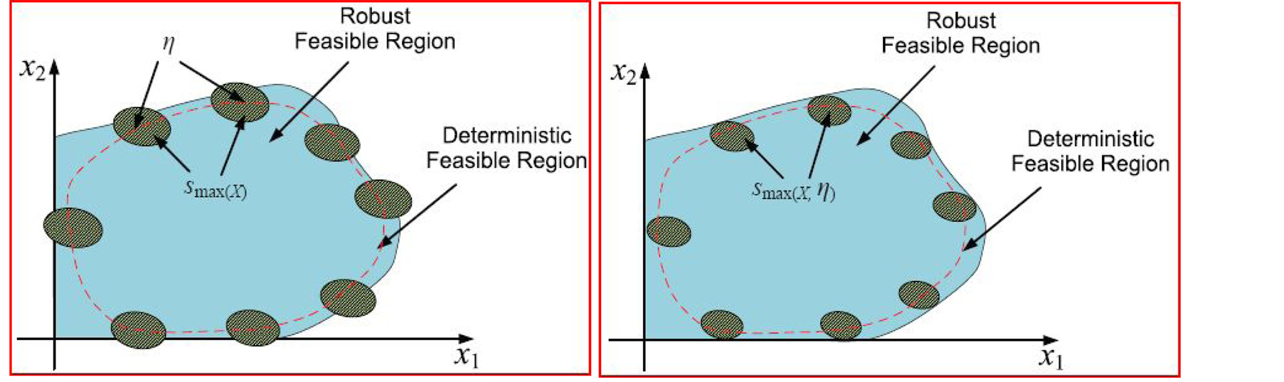
Figure 2. Robust Feasible Region with and without Budget of Uncertainty. (a) Robust feasible region at yield protection level η; (b) Robust feasible region with budget of uncertainty.
 (1.18)
where  is a scaling factor of the SOC set size for a specific yield protection level. We assume parameter variations will be enclosed by this scaled SOC set. Note that the parameter variations defined here is dependent of
 , as a result we use
  to differentiate it from the physical parameter variations
 . For simplicity we let
  in this model. Assume that the physical parameter variations obey a multivariate Gaussian distribution
  where
where  denotes the covariance matrix. We can derive that the uncertainty defined by the scaled SOC set, i.e.
  also follows a scaled Gaussian distribution:
 (1.19)
We now discuss how to approximate the scaling factor  when applying the SOC uncertainty set to the timing constraint. Applying a first-order Taylor series expansion to the probabilistic delay function yields:
 (1.20)
By substituting (1.19) into (1.20), it is possible to approximate the probabilistic constraint by a Gaussian CDF (Cumulative Distribution Function) and reveal the mapping relationship between  and
and . We start with analyzing the independent case. If the design parameters are all uncorrelated, since
 following probability theory we can derive that delay metric obeys the following Gaussian distribution:
 (1.21)
Therefore the probabilistic constraint function can be approximated as:
 (1.22)
where  is the cumulative distribution function for a standard Gaussian variable. Therefore, for a required level of yield protection, we can refer to Gaussian distribution table to find
  and further calculate the scaling factor
 .
.
For a specific yield level , we use the method described above to conduct uncertainty budgeting and obtain the optimal gate sizes satisfying yield requirement
 . Based on the gate sizing results we run Monte-Carlo simulation to determine the frequency of delay violations, i.e. the percentage that circuit delay exceeds the timing constraint
 , and compare the violation rate by uncertainty budgeting with the expected violation rate for specified
  value. The results demonstrate good accuracy of the approximation method used in budget of uncertainty.
We focus on formulating the set of constraint functions . For small parameter variations from their nominal values, the variational constraint function
  can be approximated by a first-order Taylor series expansion:
 (1.23)
where  represents the gradient of delay function
  calculated at the nominal values of gate sizes, and
  denotes the random variations around nominal gate sizes
 ’s.
’s.
From (1.23) we observe that the variational function  consists of two components: 1) the deterministic part
 , which is in signomial form; and 2) the variational part
 , consisting of a gradient term and a parameter variation term. On the other hand, all possible perturbation values in the parameter variation term are required to satisfy the timing constraint
 . In other words, the complete variational function (1.23) has to be smaller than this user-defined delay specification. This is equivalent to:
 (1.24)
which indicates that the maximum possible value of the variational function must be bounded by timing constraint . In what follows, the variational delay constraint is modeled as the deterministic constraint (1.24).
After one step of transformation, the constraint function is still not in standard GP form, and further transformations are necessary for GP formulation. We show that by employing the SOC estimation model and introducing a set of slack variables, the variational constraint function can be eventually transformed into a set of standard posynomials. The formulation procedure is applicable to delay models in form of any signomial. Posynomial delay models can be certainly addressed in the same manner since a posynomial is a special case of a a signomial.
We employ the SOC representation, which is described in Section 3, to address the parameter variation term . Given a gate size vector
  with nominal vector
 , parameter variations around the nominal values are characterized by a SOC estimation model:
 (1.25)
where  is an auxiliary parameter introduced to manipulate parameter perturbation range. The variations are considered to be bounded within the SOC region defined in (1.25), and the boundary condition
  determines the size of the SOC region. Note that
  itself is dependent on the nominal value of design parameters. As shown in (1.25),
  is a conic function of the nominal gate sizes. In addition to the linear terms of design parameters, it also includes a set of quadratic terms for the purpose of capturing the nonlinearity of the SOC size, as well as a set of cross terms for the purpose of capturing the correlations among design parameters. We have applied both linear regression and nonlinear regression techniques to fit the form of
  function (refer to the section of experimental results). The fitting results show that the assumption of conic-form
  function yields much less fitting errors and achieves good approximation accuracy.
We will show that by employing the conic-form SOC estimation model and introducing a set of slack variables, the variational constraint function can be eventually transformed into a set of standard posynomials. The formulation procedure is applicable to delay models in form of any signomial. Posynomial delay models can be certainly addressed in the same manner since a posynomial is a special case of a signomial. The robust gate sizing problem is generalized as follows:
 (1.26)
 (1.27)


The objective is already a posynomial and satisfies standard GP requirement. There are two constraints which are not in standard GP form, a robust delay constraint and the conic-form SOC constraint for uncertainty estimation. As described above, the conic-form SOC constraint (1.27) can be translated into a general-form SOC interpretation, and therefore can be accurately approximated by a set of linear constraints [24] . Further GP formulation are required. We will focus on formulating the delay constraint (1.26). We rewrite the delay function as follows:
 (1.28)
where  and
and  can be any real number. The derivative of delay function at
  is then given by:
 (1.29)
By combining the results in (1.28) and (1.29) we can express the constraint function (1.24) explicitly:
 (1.30)
where ’s represent nominal gate sizes, and
 ’s the corresponding size variations. For conciseness we do the following substitution for (1.30):

In above equation,  stands for the multiplicative coefficient and
  stands for the exponent index in posynomial delay function (1.28), therefore
  could be either positive or negative, bringing the difficulty in GP formulation since a standard posynomial does not allow negative coefficients. To address this problem, We further introduce two vectors
  to collect the positive and negative coefficients in (1.30) respectively. To be more specific, the components of vectors
  and
and  are generalized as follows:
 (1.31)
Having explained the definition of ,
,  in (1.31), we further translate (1.30) into the following expression:
 (1.32)
where  denotes the innver product of two vectors
 ![]() and
and . Following the well-known Cauchy-Schwartz inequality:
 (1.33)
an equivalent expression for (1.33) is given by:
 (1.34)
By employing the SOC estimation model and following norm properties, gate size variations can be estimated as:
 (1.35)
Substituting (1.35) into (1.34) yields the following constraint:
 (1.36)
One more step of formulation is to introduce two more slack variables  and
and ![]() to substitute
to substitute  and
and :
:
 (1.37)
Putting all the formulation results together, we conclude that the variational constraint function (1.24) has been replaced by an equivalent set of constraints:
 (1.38)
 (1.39)
 (1.40)
which is very close to a standard GP expression with the new decision variable set: . The quadratic terms in constraints (1.39) and (1.40) are already in standard posynomial form by expanding them:

Above expansion indicates that the quadratic terms both are summations of posynomials with all positive multiplicative coefficients, therefore the constraints (1.39) and (1.40) are also posynominals and they satisfy the requirements of GP formulation.
The last step is to transform the signomial constraints into posynomial constraints. [25] introduces an efficient way of such conversion. After such transformation, the final formulated GP can be efficiently solved by existing GP tools. In real application, this formulation procedure is repeated for all delay constraints, and the final formulated GP problem can be solved by convex optimization tools. It is worth emphasizing that if we take uncertainty budgeting into account, the formation of  will be dependent on not only the conic-form fitting function, but also the yield-determined size of the SOC uncertainty set.
5. Experimental Results
In this section we present the robust gate sizing results on ISCAS benchmark circuit. All simulations and experiments were performed on a quad-core 2.8-GHz machine with 4-GB memory. In simulation part, we use the 65nm technology node provided by PTM model [26] . The coefficients in gate delay functions are extracted from HSPICE simulation data. We assume 20% process variations for all gate sizes around their nominal values. An convex optimization software GPPLAB [27] was used to solve the final GP problem. The optimization
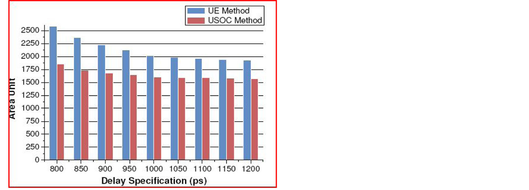
Figure 3. Area costs for C432 circuit with different delay specifications UE means Uncertainty Ellipsoidal USOC refers to the new method.
objective is to minimize the total area , where
  denotes the number of transistors in gate
 , and gate size
  stands for the ratio of area of gate
  to that of a minimum sized inverter. Figure 3 demonstrates this experimental result. We compared delay specification and area consumption of uncertainty ellipsoidal (UE) and our proposed method USOC. It can be noticed that with the same delay specification, we have 20% of reduction in area consumption.
6. Conclusion
This paper presents a novel uncertainty estimation model for robust gate sizing under process variations. The new model employs the concept of SOC to accurately characterize local variations around nominal gate sizes. With gate size variations characterized in SOC estimation, the robust gate sizing problem can be formulated into a standard geometric program, and therefore can be efficiently solved by existing GP solvers.
References
- Boning, D. and Nassif, S. (2001) Models of Process Variations in Device and Interconnect. In Chandrakasan, A., Bowhill, W.J. and Cox, F., Eds., Design of High-Performance Microprocessor Circuits, Chapter 6, IEEE Press, 98-115.
- Roy, S. and Asenov, A. (2005) Where Do the Dopants Go? Science, 309, 388-390.
- Orshansky, M., Milor, L. and Hu, C. (2004) Characterization of Spatial Intrafield Gate CD Variability, Its Impact on Circuit Performance, and Spatial Mask-Level Correction. IEEE Transactions on Semicondictor Manufacturing, 17, 2-11. http://dx.doi.org/10.1109/TSM.2003.822735
- Hargreaves, B., Hult, H. and Reda, S. (2008) Within-Die Process Variations: How Accurately Can They Be Statistically Modeled? Proceedings of ASPDAC, Seoul, 21-24 March 2008, 524-530.
- Veetil, V., Sylvester, D., Blaauw, D., Shah, S. and Rochel, S. (2009) Efficient Smart Sampling Based Full-Chip Leakage Analysis for Intra-Die Variation Considering State Dependence. Proceedings of DAC, San Francisco, 26-31 July 2009, 154-159.
- Wang, J., Das, D. and Zhou, H. (2007) Gate Sizing by Lagrangian Relaxation Revisited. Proceedings of ICCAD, 111-118.
- Ketkar, M., Kasamsetty, K. and Saptnekar, S. (2000) Convex Delay Models for Transistor Sizing. Proceedings of DAC, 655-660.
- Kasamsetty, K., Ketkar, M. and Saptnekar, S. (2000) A New Class of Convex Functions for Delay Modeling and Its Application to the Transistor Sizing Problem. IEEE Transactions on Computer-Aided Design of Integrated Circuits and Systems, 19, 779-788. http://dx.doi.org/10.1109/43.851993
- Shyu, J.M., Sangiovanni-Vincentelli, A., Fishburn, J.P. and Dunlop, A.E. (1988) Optimization-Based Transistor Sizing. IEEE Journal of Solid-State Circuits, 23, 400-409. http://dx.doi.org/10.1109/4.1000
- Cong, J., Lee, J. and Vandenberghe, L. (2008) Gate Sizing by Lagrangian Relaxation Revisited. Proceedings of International Symposium on Physical Design (ISPD), 10-14.
- Singh, J., Nookala, V., Luo, Z. and Sapatnekar, S. (2011) A Geometric Programming-Based Worst Case Gate Sizing Method Incorporating Spatial Correlation. IEEE Transactions on Computer-Aided Design of Integrated Circuits and Systems, 53, 464-501.
- Li, X., Gopalakrishnan, P., Xu, Y. and Pileggi, L. (2007) Robust Analog/RF Circuit Design with Projection-Based Performance Modeling. IEEE Transactions on Computer-Aided Design of Integrated Circuits and Systems, 26, 2-15. http://dx.doi.org/10.1109/TCAD.2006.882513
- Hsiung, K.L., Kim, S.J. and Boyd, S. (2008) Tractable Approximate Robust Geometric Programming. Optimization and Engineering, 9, 95-118. http://dx.doi.org/10.1007/s11081-007-9025-z
- Xu, Y., Hsiung, K.L., Li, X., Pileggi, L.T. and Boyd, S.P. (2009) Regular Analog/RF Integrated Circuits Design Using Optimization with Recourse Including Ellipsoidal Uncertainty. IEEE Transactions on Computer-Aided Design of Integrated Circuits and Systems, 28, 623-637. http://dx.doi.org/10.1109/TCAD.2009.2013996
- Bertsimas, D., Brown, D.B. and Caramanis, C. (2008) Theory and Applications of Robust Optimization. SIAM Review, 27, 295-308.
- Dyer, M. and Stougie, L. (2006) Computational Complexity of Stochastic Programming Problems. Mathematical Programming: Series A and B, 106, 423-432. http://dx.doi.org/10.1007/s10107-005-0597-0
- Xu, Y., Hsiung, K.L. and Li, X. (2005) Opera: Optimization with Ellipsoidal Uncertainty for Robust Analog IC Design. Proceedings of Design Automation Conference, Anaheim, 13-17 June 2005, 632-637.
- Johnson, R.A. and Wichern, D.W. (2002) Applied Multivariate Statistical Analysis. Prentice Hall, Upper Saddle River.
- Boyd, S. and Vandenberghe, L. (2004) Convex Optimization. Cambridge University Press, New York.
- Lobo, M., Vandenberghe, L., Boyd, S. and Lebret, H. (1998) Applications of Second-Order Cone Programming. Linear Algebra and Its Applications, 284, 193-228. http://dx.doi.org/10.1016/S0024-3795(98)10032-0
- Xiong, J., Zolotov, V. and He, L. (2006) Robust Extraction of Spatial Correlation. Proceedings of International Symposium on Physical Design, San Jose, 9-12 April 2006, 2-9.
- Chang, H. and Sapatnekar, S. (2003) Statistical Timing Analysis Considering Spatial Correlation Using a Single PertLike Traversal. International Conference on Computer Aided Design, ICCAD-2003, 9-13 November 2003, 621-625.
- Stein, M.L. (1999) Interpolation of Spatial Data. Springer, New York. http://dx.doi.org/10.1007/978-1-4612-1494-6
- Ben-Tal, A. and Nemirovski, A. (2000) Robust Solutions of Linear Programming Problems Contaminated with Uncertain Data. IEEE Transactions on Computer-Aided Design of Integrated Circuits and Systems, 88, 411-424.
- Chiang, M. (2005) Geometric Programming for Communication Systems. Now Publishers, Hanover.
- Nanoscale Integration and Modeling (NIMO) Group (2011) Predictive Technology Model (ptm). http://ptm.asu.edu
- Boyd, S.P. (2011) Stephen p. Boyd—Software. Website, August. http://stanford.edu/~boyd/software.html