Applied Mathematics
Vol. 3 No. 1 (2012) , Article ID: 16760 , 8 pages DOI:10.4236/am.2012.31013
Combined Algorithms of Optimal Resource Allocation
Moscow State Technical University of Radio Engineering, Electronics and Automation, Moscow, Russia
Email: str1942@mail.ru
Received October 17, 2011; revised November 19, 2011; accepted November 28, 2011
Keywords: Dynamic programming; the Pareto set; branch and bound method; the curse of dimensionality; algorithm “descent-ascent”
ABSTRACT
Under study is the problem of optimum allocation of a resource. The following is proposed: the algorithm of dynamic programming in which on each step we only use the set of Pareto-optimal points, from which unpromising points are in addition excluded. For this purpose, initial approximations and bilateral prognostic evaluations of optimum are used. These evaluations are obtained by the method of branch and bound. A new algorithm “descent-ascent” is proposed to find upper and lower limits of the optimum. It repeatedly allows to increase the efficiency of the algorithm in the comparison with the well known methods. The results of calculations are included.
1. Introduction
The problem of optimum distribution of limited resource R between n consumers was solved by R. Bellman more than 50 years ago [1]. His method of dynamic programming allows to find the optimal path (trajectory) and lead for n steps of the system from the given initial state to the final one.
While using R. Bellman’s algorithm, which became classical, the problem comes to finding the optimal trajectory, connecting nodes of a regular grid, which actually define the set of states on each step prior to the beginning of the account.
Later on other realizations of dynamic programming have been offered, where the task of regular grid of states was not necessary. At the same time as we move from the initial point to the end we consider only achievable states (points). And from all paths that lead to each state remain only the best [2,3].
The characteristic feature of traditional algorithms of dynamic programming is intensive growth of volume of calculations with growth n and R which has the name “the curse of dimensionality”.
So, if possible resource values for each consumer are not integer and on a numerical axis are irregularly located then application of traditional Bellman’s algorithm is conjugated with essential computing difficulties because of necessity of introduction small discrete and accordingly a great number of states. If number of consumers and number of possible values of resource for each of them reaches some hundreds then time needed for the decision of real problems can be unacceptable. That is why the search of more effective algorithms especially for the big dimension problem which built in multiply repeated cycle of calculation is actual. This is the purpose of this work.
2. Problem Statement
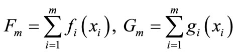
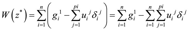
Let’s consider the following problem: to find the maximum of the sum
 (1)
(1)
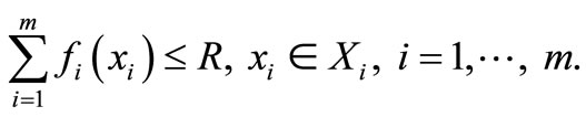
subject to
 (2)
(2)
where Xi—finite sets,  ,
,  and
and  Functions
  and
and  may not be integer. It is supposed that the set of feasible solutions (2) is nonempty.
Variety of problems which can be written in this form, comes to allocation given resource R among n consumers. Functions characterize a resource, and
 — is efficiency of it’s use. If
  and
and  we have the problem of optimum loading of vehicle objects, which weights pi, costs сi, and quantities
  [1]. If additionally
  we obtain the well-known problem of “knapsack” [2].
It might be needed to look for minimum in (1). In this case functions —a resource, and
 —expenses. For example,
 —resources of time, and
 —expenses for realization of some project.
Non-integer values of the resource arise in a problem surface protection from aggressive influence of environment [4,5]. The surface consists of n elements, for protection of each of them m various ways can be used. Their efficiency and corresponding expenses are various. In this problem, —permissible damage from incomplete protection of i-th element of surface, and
  —expenses.
The problem on maximum is reduced to an equivalent problem on minimum by replacement in (1)  on
on
 where
where .
.
Further the problem (1,2) is being considered on minimum and the following designations are used:  —values
  and
and —the corresponding values of the functions
  and
and .
.
3. Algorithms with Elimination of States
Efficiency of dynamic programming can be essentially increased by elimination not only the paths leading to some state, but also actually unpromising states which obviously can’t belong to an optimum trajectory, that is optimum sequence of states.
For the simple knapsack problem, this idea of elimination of the states is realized [2].
The algorithms realizing this idea for the decision of a more general problem (1,2), we’ll consider a problem on minimum.
 we’ll number so that
  . If
. If , then we eliminate
  if
if , and we eliminate
  if
if .
.
However the pair  can be eliminated if
  and
and as bigger resource should correspond smaller expense in the problem on minimum. In this case
  will be always used instead of
 . After elimination we get
  . Hence for any i the remained points with coordinates
  form Pareto set on a plane
 , all other variants are unpromising.
At each step of dynamic programming by the state we mean total resource, which already was used. Accordingly after the first step the set of states  is such that pairs
  form Pareto set.
At each following step  we’ll consider set of points
  of the following
where vector  runs all values, satisfying the conditions
 .
.
Let for two points  and
and  where the bottom index is number of a step, and top index is point number , we have :
 . A path
  corresponds to point
  and to point
  corresponds
 .
.
Point  can be excluded from consideration because path
  can not be a part of optimal trajectory. In fact, let
  be optimum continuation from point
 , which expenses G* correspond. Then for trajectory
  And point
  is eliminated.
 At
At  and
and  the point
  can also be excluded. It means that from the set of points
  on each step m it is possible to leave only Pareto subset, and from two congruent points remains only one. This rule also includes elimination of inefficient paths which lead to the same state, and elimination of actually unpromising states to which non Pareto points correspond.
Pareto subset of  will be designated by
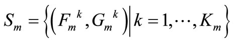 , numbering them according to increasing resource, i.e.
 . Formation of step-by-step ordered Pareto sets Sm сan be achieved in different ways. A variant where at first we form the whole set of admissible points and then leave only Pareto points turned to be ineffective. The algorithm has been realized:
The first step.
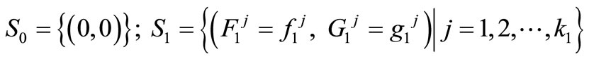 .
.
No elimination.
The general step. Assume that the set
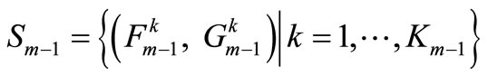
is already constructed. At first stage (k = 1) we calculate
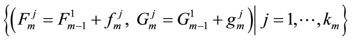
without elimination. At second stage for  (the external cycle) we consistently calculate
  (an internal cycle). May be only three results of comparison each calculated point P with already available (the nearest on value of a resource):
1) P is not included in formed set as there is a dominating point in it;
2) P is included (with reserving the order) as there is no dominating point in relation to it, and it isn’t dominating;
3) New point P is included in the formed Pareto set, and one or probably more points in relation to them P is dominating, are eliminated from it.
Owing to orderliness Pareto set and  no necessity to analyse all points for search a dominating point. At k = 2 and j = 1 search begins with 1, i.e. points with
 . At
. At  and j = 1 search begins with number received by a point with
  or dominating over it. At
  and
and  search in an internal cycle begins with number, received by point with
  or dominating over it. Search goes always with increase of resource and comes to an end at achievement
 , i.e. the resource of the new point—“candidate”. In item 3 search of dominated points begins with N + 1 where N—number of the new point which was included and stops at the first unsuccessful attempt.
As a result we receive Pareto set of points, which are ordered on increase of a resource.
For problems of big dimension the number of Pareto points can be great, especially at non integer values  that has demanded working out of the new algorithms, allowing to eliminate some unpromising Pareto points. It is possible on each step of dynamic programming if to use the approximate decision (initial approach) as the top estimation of optimum with possibility of its clarification in the process of the account or to build bilateral prognostic estimations of optimum. In particular on each step Pareto set include points corresponding minimum resources and accordingly maximum expenses which through some steps can already exceed total expenses for all steps, corresponding to initial approach. Such situation comes for smaller number of steps in the presence of good initial approach.
Let’s assume that some admissible vector  is calculated and the corresponding value of the target function is
At the decision of a problem (1,2) on minimum on a step m Pareto point  is eliminated, if
 , as it can’t belong to optimum trajectory because on subsequent steps target function can increase only as
If for  and a value
  , then
  is non Pareto point. It is replaced on
 ; for
; for  we remain
  (accordingly
  and
and ), therefore all
  we decrease on δ, and
 we decrease on
 .
.
On subsequent steps  corrected values
  and
and  are used for elimination Pareto points. Expenses for the rest part of a trajectory and accordingly the top border of total expenses can be calculated approximately for everyone Pareto point. We decrease
 , using minimum of received values of total expenses, and receive an opportunity of additional elimination Pareto points. Correspondent algorithms use obtained values
  as the top estimations of optimum, and the bottom estimation is equal to zero and, as a rule, it is far from optimum.
We use a combination of dynamic programming and a method of branches and borders for construction the improved bilateral estimations of optimum. Thus everyone Pareto point on each step is considered as a point of branching with construction of bilateral estimations of optimum (the bottom and top border). Efficiency of such method depends on quantity of states, computing expenses for borders calculation and their nearness to optimum.
Let’s designate expenses for all trajectory, corresponding to initial approach, through E (in a method of branches and borders they are called as a record), and their bottom border through H. Expenses for the rest part of trajectory from a point , corresponding to some admissible approach, we will designate through
 , their bottom border through
 . Then condition of elimination Pareto points
  will become
  . If
. If , new value of a record is
 . We modify initial approach accordingly.
If for some m and j  there is no sense to consider
 , as a branching point. If additionally
  this point and corresponding trajectory are remembered and stored until then yet won’t be obtain value of a record smaller, than
 . If “the record will stand” then corresponding decision is optimum. If on some step there will be no Pareto points the record is the required decision. On each step it is possible to correct the bottom border, replacing H on

and to stop calculation at where ε is defined by demanded accuracy of the decision.
4. Construction of Initial Approach (The Top Border)
The simple algorithm of construction of initial approach consists in the following steps:
1) For  consecutive for
  it is postponed
  on an axis of abscisses, and
  on an axis of ordinates and we receive sequence of points, which defines strictly monotonously decreasing piecelinear function, because
  are Pareto points. We will consider that such functions are constructed for all i.
2) We calculate  and
and .
.
If , the problem has no decision. If
 , we have the trivial decision, choosing
  for everyone i. Let’s designate
 . We make
 .
.
3) We calculate . If
. If  ,then we make
 , further we eliminate i from I, replace k on k − 1, R on
  and repeat item 3, differently
  and we go to item 4.
4) For  we consistently define
  and replace
  on
on . Accordingly
 .
.
5) Initial approach (trajectory)
Similarly, it is possible to build initial approach in the process of dynamic programming for the rest part of the trajectory, starting with any Pareto point.
5. Calculation of Bilateral Estimations of an Optimum
For construction of bilateral estimations of an optimum we use the piece-linear functions received in item 1. Those of them which aren’t convex, we will replace on their convex shells . As a result we receive a continuous estimated problem: to find a minimum
 (3)
(3)
and
 (4)
(4)
Optimum of a continuous problem (3,4) which it is obvious no more an optimum of a problem (1,2), we will accept as required bottom border.
In this problem of nonlinear programming the target function and the system of restrictions have essential features which will be used for its decision by simple algorithm.
The ends of links of broken lines wi(zi) we will designate through  (j = 1, ···, pi).
We have , if
, if — convex function, differently
 . Values
we will name biases. Owing to monotony and convexity functions  sequence of biases
  is strictly monotonously decreasing.
The problem (3,4) has simple sense: it is how much necessary to go down on each broken line  from the initial point that without breaking restriction on the sum of abscisses, to receive the minimum sum of ordinates? The simple and obvious enough answer:- on each step it is necessary to go down along a link with the maximum bias. We will result a formal substantiation of this statement.
Let —the decision of a problem (3,4). We will designate through
 —a set of all biases,
 ,
,

and
—accordingly sets of the biases completely used for descent, used partially and not used at descent.  .
.  for
for 
 (5)
(5)
where , if
, if ;
; , if
, if  and
and , if
, if .
.
Let . We will prove that
 , respectively
 .
.
Let’s assume that this statement isn't true. We take the minimum bias , to it corresponds
  Having reduced
  by some Δ, we receive target function increase on
  and possibility of its reduction by the big value
  without violating restriction on the resource, as
 . Hence
  not an optimum. The received contradiction proves necessity of use of the maximum bias. Necessity of whole using of the maximum from unused biases is similarly proved, the resource won’t be settled yet.
As a result we receive the following algorithm of descent:
1) We take initial point , which corresponds the maximum value of target function
We fix the rest of resource 
2) From all links of all broken lines we take a link with the maximum bias. Let it will be a link with number j of a broken line with number m. On the first step j = 1 owing to convex and monotony of broken lines. We will change only a variable zm. Its increase gives reduction of target function with the greatest speed. We calculate a movement step  and replace
  on
on . Target function will decrease on
 , and the remained resource will decrease on c.
3) From all remained links of all broken lines we choose again a link with the maximum bias and repeat item 2 while remained resource T won’t be settled.
If there are several links with the maximum bias the priority is given to a link with the maximum length which the remained resource allows to use completely . If a resource is not enough for full use of any of such links, any of them is used.
Let’s notice that in a minimum point only bias , which used by last, can be used partially. If it also is used completely, i.e. on last step
 , the received decision of continuous problem coincides with the decision of initial discrete problem and it is definitive. Otherwise it is initial approach, and value of target function in a minimum point is required bottom border H0. If last considered a broken line initially was convex
  we receive the approached decision of initial discrete problem and accordingly record E by canceling last step (it explains the aspiration to make it less). Otherwise we define the absciss of the node nearest at the left on broken line
  using optimum value
 . Ordinate of this node, we will designate through
 . The bottom border H0 doesn’t change, and record
  .
.
Note that convex shells are used only to calculate the borders, but at formation of a set of states on each step, we consider all admissible states, i.e. initial broken lines.
For effective realization of the algorithm essential value has a way of search of the greatest biases. The simple way consists in sorting of all biases of all links of all broken lines. But expenses of operative memory for sorting can be excessive as the essential part of biases in general can not be demanded at calculation of the bottom border and a record. Instead of complete sorting only biases of the first elements of broken lines are ordered as it should be nonincreasing. With each of them number of a broken line and number of its link communicates. Initial number of its link is equal 1. In the presence of equal biases the priority is given to a link with the greatest length. The received array of biases we will designate through . According to the stated algorithm descent process begins with use
  and continues with maximum biases. Further, if the current bias is used completely it is replaced in the array U on
 , i.e. bias of the next link of the same broken line maintaining order in the array U. If we can not completely use the next bias because of the restriction on resource, it is used partially and the descent is finished.
On the first step  and
and , where
  . The bias
  is located in the array U so that the condition not increasing of its elements was satisfied. If
  , the elements of U more than
 , move to the left, so on the first place always stands the greatest bias. If all links of some broken line s were used, the fictitious link with number
  and a zero bias is entered, and process proceeds before resource exhaustion. The total array of biases, and also
 , that is a part of a link of a broken line which was used by the last at descent is remembered.
Alternative to algorithm of descent is ascent from a point  with the minimum value of target function
 , which increases on each step with a minimum speed because we use the next minimum bias. The used resource decreases from
  to R. In this algorithm in case of exhaustion of all biases (links) of some broken line the fictitious link with number a zero is entered. Its bias is equal to a great value.
As a result we receive and remember the new array of biases , and also
 —a part of a link of a broken line which was used by the last at ascent. Both algorithms give the same decision
  and value of target function (the bottom border H0), but arrays of biases U and V are different. In the array U—biases of links—applicants for the further descent, and in the array V—on ascent. Everyone i-th broken line is presented by a bias of one link, but number of this link in array U one more, as
  is equal to an absciss of the left end of the link presented in the array U or the right end in the array V. The exception is made by the broken lines presented by biases, appeared as a result on the first places
  and
and .
. , with them the same j-th link of a broken line is connected. This line was used by the last. Its number is s, thus
  .
.
The algorithm of ascent is proved similarly as the algorithm of descent. It begins to work with ranking in order of decreasing biases of last links of all broken lines.
The algorithm of descent can be also used for calculation of borders of expenses on the rest part of a trajectory for everyone Pareto point.
Let’s note two features of this algorithm:
1) An array of n biases received as a result and the data connected with it about numbers of broken lines and their links contains the necessary information for decision restoration z* and corresponding optimum trajectory for a continuous problem (sequence of states  ).
).
2) If instead of R we have  there is no sense to begin descent anew, it can be continued from received for R an optimum point, using a total array and the remained biases. However at
  for updating of the received decision we are forced to descend anew.
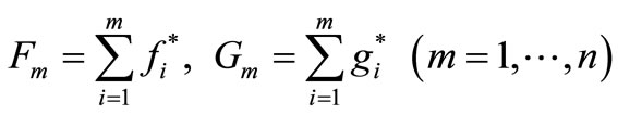
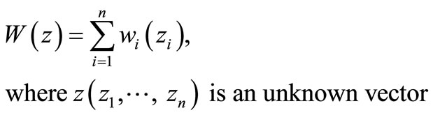
3) If from a total array exclude all biases, which concern the first broken line, then the resulting array will correspond the decision  of a problem:
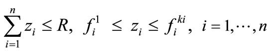
 , where
 —an unknown vector, at restrictions
 because for decision of this problem it should to use the maximum biases from all broken lines, except the first. In other words, the resulting array of biases corresponds to an optimum trajectory from a state which was received after the first step of algorithm
  up to the end.
Similarly, passing to the next r-th step of algorithm of dynamic programming and excluding from array U biases , we receive the array of biases, which corresponds
  and therefore to a state
  on an optimum trajectory.
It is similarly possible to use the algorithm of ascent.
Essential lacks of the stated algorithms of descent and ascent are:
1) Initial points are far from an optimum.
2) Information about the optimal trajectory, which was found on the first step in solving the continuous problem, is not used.
3) As a rule, new values of a record turn out for the points located near to a point on an optimum trajectory. But these algorithms find a new value of a record already after points which could be eliminated at movement from a point on an optimum trajectory were passed.
New algorithm of calculation of borders which we name “descent-ascent” is free from these lacks. Its basic points:
1) The initial estimated problem (3,4) is solved both a method of descent and a ascent method. Arrays U and V, as base, and also Δb and Δb1 are remembered. Each element of each array connected with number of a broken line and number of a link to which it corresponds. That gives the chance to restore the optimum point z* and the optimum trajectory.
2) The optimum trajectory  and corresponding borders E0 and H0 are remembered. This is decision of an estimated problem, and a deviation from an optimum of an initial problem doesn’t exceed
 .
.
3) We construct Pareto set after the first step of dynamic programming.
4) The biases corresponding to the first broken line are excluded from arrays U and V.
5) Starting with state  descent for states with
 , and ascent for states with
  are carried out consistently for definition of bottom and top border costs for the remainder of the trajectory and possible elimination of a state or record updating.
6) On the subsequent steps of dynamic programming both borders are defined similarly.
Special is s-th step of algorithm of dynamic programming, where s is a number of a broken line to which posesses a link used by last at construction of an optimum trajectory of a problem (3,4). Its bias was used partially, therefore at removing of this bias from base arrays of biases, Δb and Δb1 are nulled.
In aforementioned special cases of a considered problem all calculations become simpler, as at  and
and  for everyone a broken line all links have one bias, and at
  each broken line consists of one link.
As the algorithm of descent-ascent demands considerable volume of calculations, for revealing of its efficiency in comparison with more simple algorithms experimental calculations have been executed.
6. Experimental Calculations
To compare the different algorithms they were implemented in the next computer programs:
P1—Dynamic Programming with elimination of the path which lead to the same state;
P2—Elimination only nonPareto states;
P3—Additional elimination of a part unpromising Pareto states with use initial approach;
P4—Additional elimination unpromising Pareto states with calculation of the bottom and top borders of an optimum on algorithm of descent-ascent.
Calculations were carried out on personal computer Intel Pentium 4, CPU 3.0 GHz, 512 MB the RAM.
In calculations abscisses and ordinates of broken lines are pseudo-casual real numbers from [1,100], but the number of tops of broken lines  didn’t depend from i.
Account time depends not only on number of steps n, value of K and from a preset value of resource R, but also from concrete values  and
and .
.
In the first calculation small values n = 50 and K = 10 were set. Results are presented in table 1. Designations: sum—total number of remembered states on all steps, max—maximum number of states on a separate step, T—time of the account in seconds.
Calculations on P1 were carried out under an additional condition: states on each step are considered coinciding if they differ (on a resource) less, than on the set
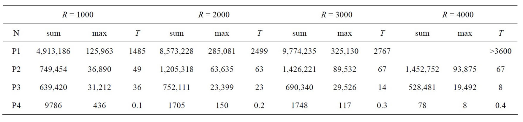
Table 1. Calculations with n = 50 and K = 10.
value d.
Attempt to receive result with d = 0.001 was unsuccessful because of excessive for-expenditure machine time. In the table the result received at d = 0.005 is presented. At d = 0.01 account time was essentially less, but accuracy of calculation can appear insufficient as on deviation target function exceeded 0.1.
Calculations under other programs were satisfied without this additional condition, but at comparison of real values the constant 10−9 was used.
Account time on P4 was less than 0.1 sec, and at R = 4000 the account has come to the end on 30th step. It is interesting a sudden reduction of account time on P3 with increasing R. In this calculation on P3 uniform distribution of a resource between consumers appears more close to an optimum with increasing resource R as the maximum requirements for a resource at consumers differ slightly.
In further calculations program P1 wasn’t used because of hopelessness of algorithm for a considered class of problems. The classical algorithm of dynamic programming (a method of a regular grid) is especially unpromising at a grid step d, equal to the value used at work with P1.
Essential influence on growth of time of the account renders growth K. So at n = 40 and K = 20 already at R = 2500 and use P2 sum = 2,748,038, max = 200,040, T = 809 sec, and at use P3 sum = 1,433,853, max = 81,889, T = 241 sec. At increase R the number remaining Pareto points becomes unacceptably big. There is a same situation, as with algorithm P1: operative memory is exhausted, and exchange with connected external memory is slow. It is characteristic that in the same calculation on P4 at R = 2500 sum = 2886, max = 152, T < 0.5 seconds, but at R = 1000 P4 gives sum = 6855, max = 500 and T = 1.2 second.
Similar results have been received under the same conditions, but with n= 100 and K = 40. The decision on P2 and P3 during comprehensible time managed to be received only at d = 0.002 and more. So at R = 2000 and d = 0.005 P3 gives sum = 7,367,886, max = 98,087 and T = 3208 sec. And at use in this calculation P4 increase R gave both increase, and reduction of number of the points which have remained after elimination. Accordingly account time both increase and reduce. Results are presented in table 2.
It is characteristic that in this calculation small change of R has essentially affected on account time. It is visible from table 3.
We explain the received results that at R = 2077 initial value of a record differs from an optimum on 0.29, and at R = 2078 on 0.34. As appears from resulted above algorithm, with increase R value of a bias  which at calculation of initial values of bottom border H0 and record E0 is used by the last, can only decrease. It gives smaller value
 , if
, if  is constant because
  . Here
 —an absciss of the point received at descent on a link of a broken line with number s at calculation H0, and
 —an absciss of the top of this broken line nearest at the left, used at calculation E0, that is at “rounding off” to the decision of a discrete problem. But reduction
  can be compensated by difference increase
 , which can both to increase, and to decrease with growth R that depends on the initial data
 .
.
For revealing of possibilities of use P4 for the decision of problems of the big dimension calculations have been executed at K = 20 and n = 100, 200, 300, 400, 500. It is established that the number of remembered states and accordingly account time essentially depends from R. So at n = 400 and R = 28,000 sum = 108,893, max = 1099 and T = 2 sec. And at R = 2000 only in the same conditions sum = 544,554, max = 3335 and T = 1189 second. At n = 500 and R = 35,000 sum = 222475, max = 1740 and T = 12 second.
In general the increase n and K doesn’t mean obligatory growth of time of the account as at “successful” R that is at small  this time can be a little and in problems of the big dimension. At any initial data exists R at which initial approach appears the final decision
  For this purpose it is enough to repeat calculation, having reduced R on
  or having increased R on
 .
.
If at use P4 to be limited to approximate solution, for example instead of d = 10−9 use d = 10−5, then in the same conditions the number of states and account time
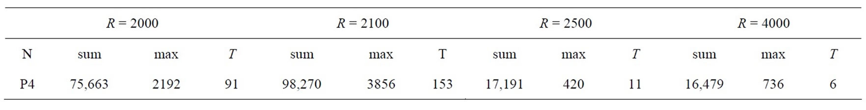
Table 2. The decision on P4 with various R.
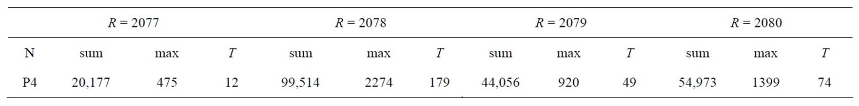
Table 3. The impact of small change of R on account time.
essentially decreases. However more perspective appears the termination of account when  instead of increasing d.
If e = 10−5 in any of calculations, which were discussed above, the account time on P4 did not exceed 0.5 sec.
Thereupon problems with n = 4000 and K = 40, and then with n = 5000 and K = 50 in the same conditions of a choice  have been solved. At R = 105,
  and
and  and e = 10−5 account stopped after the third step, and time of the account didn’t exceed 8 seconds. Similar results have been received and at a casual choice
  from [1,1000], preservation of all other parameters of calculation and at various values R.
In addition as an option in the program P4 descent algorithm was used in place of the descent-ascent algorithm. It is established that the descent algorithm in all the calculations required more time than the algorithm of descent-ascent. Moreover, the computing time on a P4 with descent algorithm in some calculations was greater than P3, because of the limitations descent algorithm noted above.
7. Conclusions
The results of comparison between different algorithms (P1, P2, P3, P4) leads to the following conclusions:
1) For the decision of problems (1,2) classical algorithms of dynamic programming can be considered as become outdated.
2) The most perspective is the combined algorithm (P4).
3) At use of the combined algorithm it is expedient to search for the approximate solutions, breaking the account at small a relative error of search of minimum e. For this purpose it is possible to set acceptable value e, but instead for the decision of problems of the big dimension it is possible to set obviously small e, to display step-by-step values E, H and  and finish process taking into account current results and elapsed time.
4) At growth R and n it is possible both increasing, and decreasing of account time. Actually algorithm P4 if doesn’t overcome completely “a dimension damnation” does its action selective.
The problem (1,2) is considered as an example, but the algorithms using Pareto sets, although not universal, as well as dynamic programming at whole, are applicable and for the decision of other problems: a various kind two-parametrical problems of distribution of resources, storekeeping, calculation of plans of replacement of the equipment, a choice of suppliers and so on.
High-speed algorithm descent-ascent can be used to solve the problem of the form (1.2), in which there are several restricts (2). This more complicated problem is reduced to a multiple solution of (1,2) with one restriction.
Consideration of these problems is beyond of the present article.
REFERENCES
- R. Bellman and S. Drejfus, “Applied Dynamic Programming,” Princeton University Press, Princeton, 1962.
- S. Martello and P. Toth, “Knapsack Problems: Algorithms and Computer Implementation,” John Willey & Sons Ltd., Chichester, 1990.
- S. Dasgupta, C. H. Papadimitriou and U. V. Vazirani, “Algorithms,” McGraw-Hill, Boston, 2006.
- V. I. Struchenkov “ Dynamic Programming with Pareto Sets,” Journal of Applied and Industrial Mathematics, Vol. 4, No. 3, 2010, pp. 428-430, doi:10.1134/S1990478910030154
- V. I. Struchenkov. “Optimization methods in applied problems,” Solon-Press, Moscow, 2009.