Communications and Network
Vol.5 No.4(2013), Article ID:40159,10 pages DOI:10.4236/cn.2013.54046
Lossless Compression of SKA Data Sets
Department of Electrical Engineering, University of Cape Town, Cape Town, South Africa
Email: karthik.rajeswaran@uct.ac.za, simon.winberg@uct.ac.za
Copyright © 2013 Karthik Rajeswaran, Simon Winberg. This is an open access article distributed under the Creative Commons Attribution License, which permits unrestricted use, distribution, and reproduction in any medium, provided the original work is properly cited.
Received October 17, 2013; revised November 12, 2013; accepted November 20, 2013
Keywords: Square; Kilometre; Array; Lossless; Compression; HDF5
ABSTRACT
With the size of astronomical data archives continuing to increase at an enormous rate, the providers and end users of astronomical data sets will benefit from effective data compression techniques. This paper explores different lossless data compression techniques and aims to find an optimal compression algorithm to compress astronomical data obtained by the Square Kilometre Array (SKA), which are new and unique in the field of radio astronomy. It was required that the compressed data sets should be lossless and that they should be compressed while the data are being read. The project was carried out in conjunction with the SKA South Africa office. Data compression reduces the time taken and the bandwidth used when transferring files, and it can also reduce the costs involved with data storage. The SKA uses the Hierarchical Data Format (HDF5) to store the data collected from the radio telescopes, with the data used in this study ranging from 29 MB to 9 GB in size. The compression techniques investigated in this study include SZIP, GZIP, the LZF filter, LZ4 and the Fully Adaptive Prediction Error Coder (FAPEC). The algorithms and methods used to perform the compression tests are discussed and the results from the three phases of testing are presented, followed by a brief discussion on those results.
1. Introduction
Astronomical data refer to data that are collected and used in astronomy and other related scientific endeavours. In radio astronomy, data that are collected from radio telescopes and satellites are stored and analysed by astronomers, astrophysicists and scientists. Digital astronomical data sets have traditionally been stored in the Flexible Image Transport System (FITS) file format, and are very large in size. More recently, the Hierarchical Data Format (HDF5) has been adopted in some quarters, and it is designed to store and organize large amounts of numerical data, as well as provide compression and other features.
With the size of astronomical data archives continuing to increase at an enormous rate [1], the providers and end users of these data sets will benefit from effective data compression techniques. Data compression reduces the time taken and the bandwidth used when transferring files, and it can also reduce the costs involved with data storage [2].
The SKA Project
The MeerKAT project, which involves a radio telescope array to be constructed in the Karoo in South Africa, is a pathfinder project for the larger Square Kilometre Array (SKA) [3]. Once the MeerKAT is complete, it will be the world’s most powerful radio telescope and provide a means for carrying out investigations, both in terms of astronomical studies and engineering tests, facilitating the way towards the efficient and successful completion of the SKA.
The SKA will allow scientists to explore new depths of the Universe, and it will produce images and data that could be in the order of Petabytes (PB) of size [4].
A software environment is used to analyze and extract useful information from these pre-processed data sets, which are used by scientists and astrophysicists. Improving the performance and functionality of this software environment is one of the main focus areas of research being conducted as part of the MeerKAT project.
Previous studies have discussed the big data challenges that would be faced by large radio arrays [5] and have explored the signal processing [1,6] and data compression techniques [7] that are used in analyzing astronomical data.
2. Objectives
The requirements and objectives for this study stem from meetings with members of the Astronomy Department at the University of Cape Town and with the chief software engineers working on the SKA project. The meetings helped to gain a better understanding of how this project would benefit the end users (astrophysicists and scientists), and how it would reduce storage costs and allow faster access to the data sets for the SKA project.
The SKA project has a custom software environment used to process and extract information from HDF5 files. The HDF5 file format has a well-defined and adaptable structure that is becoming a popular format for storing astronomical data.
The main focus of this project was to compress the total size of the files containing the astronomical data without any loss of data, and do this while streaming the data from the source to the end user. This main objective has been divided into the following research goals:
1) Investigate and experiment with different data compression techniques and algorithms;
2) Find the optimal data compression algorithm for the given data sets;
3) Attempt to implement the algorithm while streaming the data sets from a server;
4) Demonstrate the algorithms functionality by testing it in a similar environment to the SKA as a stand-alone program.
3. Background
3.1. Astronomical Data in Radio Astronomy
Astronomical data refers to data that is collected and used in astronomy and other related scientific endeavours. In radio astronomy, data that is collected from radio telescopes and satellites is stored and analysed by astronomers, astrophysicists and scientists [1]. Digital astronomical data sets have traditionally been stored in the FITS file format, and are very large in size [8]. More recently, the Hierarchical Data Format (HDF5) has been adopted in some quarters, and is designed to store and organize large amounts of numerical data.
The invention and commercialization of CCD data volumes has led to astronomical data sets growing exponentially in size [9]. (Figure 1) below provides evidence of this, showing how astronomical data has grown in size from the 1970s. These results were obtained from a study carried out on the LOFAR project, which is a pathfinder to the SKA.
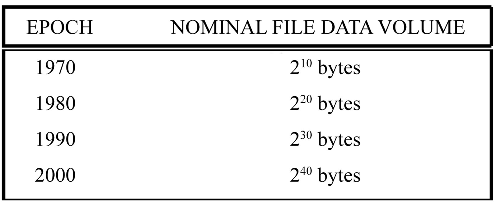
Figure 1. Increasing bit size of astronomical data [10].
Most astronomers do not want to process and analyze data and have to delete it afterwards. Variable astronomical objects show the need for astronomical data to be available indefinitely, unlike Earth observation or meteorology. The biggest problem that arises from this situation is the overwhelming quantity of data which is now collected and stored [1].
Furthermore, the storage and preservation of astronomical data is vital. The rapid obsolescence of storage devices means that great efforts will be required to ensure that all useful data is stored and archived. This adds to the necessity of using a new standard to overcome the potential break down of existing storage formats [11].
3.2. The HDF5 File Format
The Hierarchical Data Format (HDF) technology is a library and a multi-object file format specifically designed to transfer large amounts of graphical, numerical or scientific data between computers [12]. HDF is a fairly new technology and was developed by the National Centre for Supercomputing Applicaionts (NCSA), while the HDF Group currently maintains it. It addresses problems of how to manage, preserve and allow maximum performance of data which have the potential for enormous growth in size and complexity. It is developed and maintained as an open source project, making it available to users free of charge.
HDF5 (the 5th iteration of HDF) is ideally suited for storing astronomical data as it is [13,14]:
• Open Source: The entire HDF5 suite is open source and distributed free of charge. It also has an active user base that provides assistance with queries.
• Scalable: It can store data of almost any size and type, and is suited towards complex computing environments.
• Portable: It runs on most commonly used operating systems, such as Windows, Mac OS and Linux.
• Efficient: It provides fast access to data, including parallel input and output. It can also store large amounts of data efficiently, has built-in compression and allows for people to use their own custom built compression methods.
3.3. Data Compression Algorithms
Data compression algorithms determine the actual process of re-arranging and manipulating the contents of files and data to reduce their size. Golomb coding and Rice Coding are two of the most commonly used algorithms, and serve as the basis for numerous compression techniques.
The following were found to be the best performing algorithms for the given HDF5 files.
3.3.1. SZIP
SZIP is an implementation of the extended-Rice lossless compression algorithm. The Consultative Committee on Space Data Systems (CCSDS) has adopted the extended-Rice algorithm for international standards for space applications [15]. SZIP is reported to provide fast and effective compression, specifically for the data generated by the NASA Earth Observatory System (EOS) [16].
SZIP and HDF5
SZIP is a stand-alone library that is configured as an optional filter in HDF5. Depending on which SZIP library is used, an HDF5 application can create, write, and read datasets compressed with SZIP compression, or can only read datasets compressed with SZIP.
3.3.2. GZIP
GZIP, is a combination of LZ77 and Huffman coding and is based on the DEFLATE algorithm. DEFLATE was intended as a replacement for LZW and other data compression algorithms which limited the usability of ZIP and other commonly used compression techniques.
3.3.3. LZF
The LZF filter is a stand-alone compression filter for HDF5, which can be used in place of the built-in DEFLATE or SZIP compressors to provide faster compression. The target performance point for LZF is very highspeed compression with an “acceptable” compression ratio [17].
3.3.4. PEC
The Prediction Error Coder (PEC) is a highly optimized entropy coder developed by researchers at the University of Barcelona in conjunction with the Gaia mission, which is a space astrometry mission of the European Space Agency (ESA) [18]. The PEC is focused on the compression of prediction errors, thus a pre-processing stage based on a data predictor plus a differentiator is needed. It is a very fast and robust compression algorithm that yields good ratios under nearly any situation [13].
FAPEC
The FAPEC (Fully Adaptive Prediction Error Coder) is a fully adaptive model of the PEC, meaning that it automatically calibrates the necessary settings and parameters based on the type of data that needs to be compressed.
It is a proprietary solution commercialized by DAPCOM Data Services S.L., a company with expertise on efficient and tailored data compression solutions, besides data processing and data mining. The company offers not only this efficient data compression product, applicable to a large variety of environments, but also the development of tailored pre-processing stages in order to maximize the performance of the FAPEC on the kind of data to be compressed.
3.3.5. LZ4
The LZ4 algorithm was developed by Yann Collet and belongs to the LZ77 family of compression aglorithms. Its most important design criterion is simplicity and speed [19].
4. Methodology
The data collected from the SKA will be stored in huge data centres, from which various end users will access the data. It was initially proposed that the compression should occur while the data is stored at the server end (as soon as it is collected), before the end user can access it (Figure 2).
This was modified at a later stage, with the compression to occur while the files were being read from the server, which is in line with the third objective of the project.
The intention was for the compression algorithm to be assimilated into the software stack that the SKA currently has in place. An additional functionality was that it should work as a stand-alone program.
From discussions with the SKA, the main priority with regards to the compression of the data was the compression ratio, with compression time and memory usage coming next. It was also mentioned that all of the data contents must be preserved, including any noise, making the compression lossless. Thus, two main stages of test-
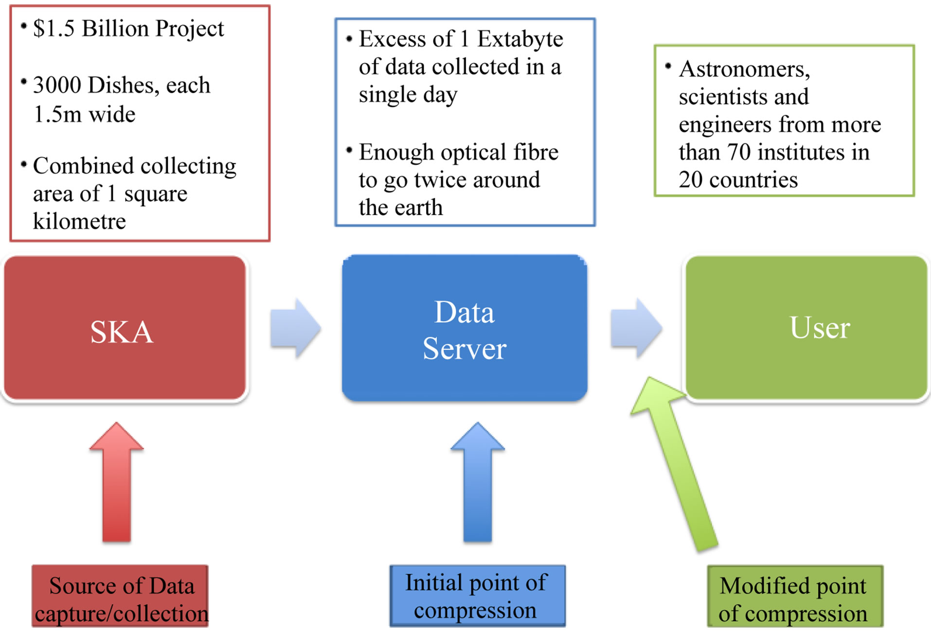
Figure 2. Image showing the process of data capture, storage and consumption (Adapted from [20]).
ing were carried out:
1) Compressing the entire data set and attempting to obtain as the highest possible compression ratio;
2) Modifying and using different parameters within the algorithms to opitmize their performance and obtain the best results.
Various algorithms were investigated and considered, with the following 5 being chosen for use in the testing process based on the compression ratios and speeds they provided for the given data sets.
1) GZIP 2) SZIP 3) LZF 4) FAPEC 5) LZ4 The algorithms were evaluated as follows:
• Each algorithm was run on data sets of different sizes, across a wide range (30 MB to 9 GB).
• The compression ratio and time taken were recorded for each test.
• The results from these tests helped to determine which algorithm/technique was the best for the given astronomical data sets.
• Compression was applied while the data sets were streamed from the server to the user, simulating the SKA environment.
5. System Design and Testing
The testing system was comprised of the:
• Testbeds—Computers and software used for testing
• Datasets—Files collected from SKA to be tested on
• Compression techniques—Techniques used to compress datasets on the testbeds The different compression techniques were installed on the testbeds. When the datasets were loaded or read, the testing environment was activated and the algorithms were run on the files being tested. The achieved compression ratio, time taken and memory used (in certain scenarios) then formed the results for this project (Figure 3).
5.1. Testbeds
The testbeds consisted of the computers, and the software applications and tools on them that were used to run and test the performance of the different compression techniques on the datasets.
In order to obtain relevant results, it was necessary to attempt to simulate the computing environment used by the SKA. This included:
• Computers running Linux-based operating systems—The majority of the machines at the SKA run versions of the Ubuntu operating system. Given that Ubuntu is open source and that the researcher had previous experience using it, it was chosen as operating system to use.
• h5py Interface—The h5py interface is a python module designed for the HDF5 format. It allows users to easily access and manipulates HDF5 files using python commands.
• Streaming files from a server—This involved streaming the datasets from another computer (which acted as the server) and attempting to compress them as they were being read.
A main computer (primary testbed) was used to run the compression algorithms, while a second machine (server testbed) was used to host and send the data when re-creating the streaming environment. This machine had the same specifications as the main computer.
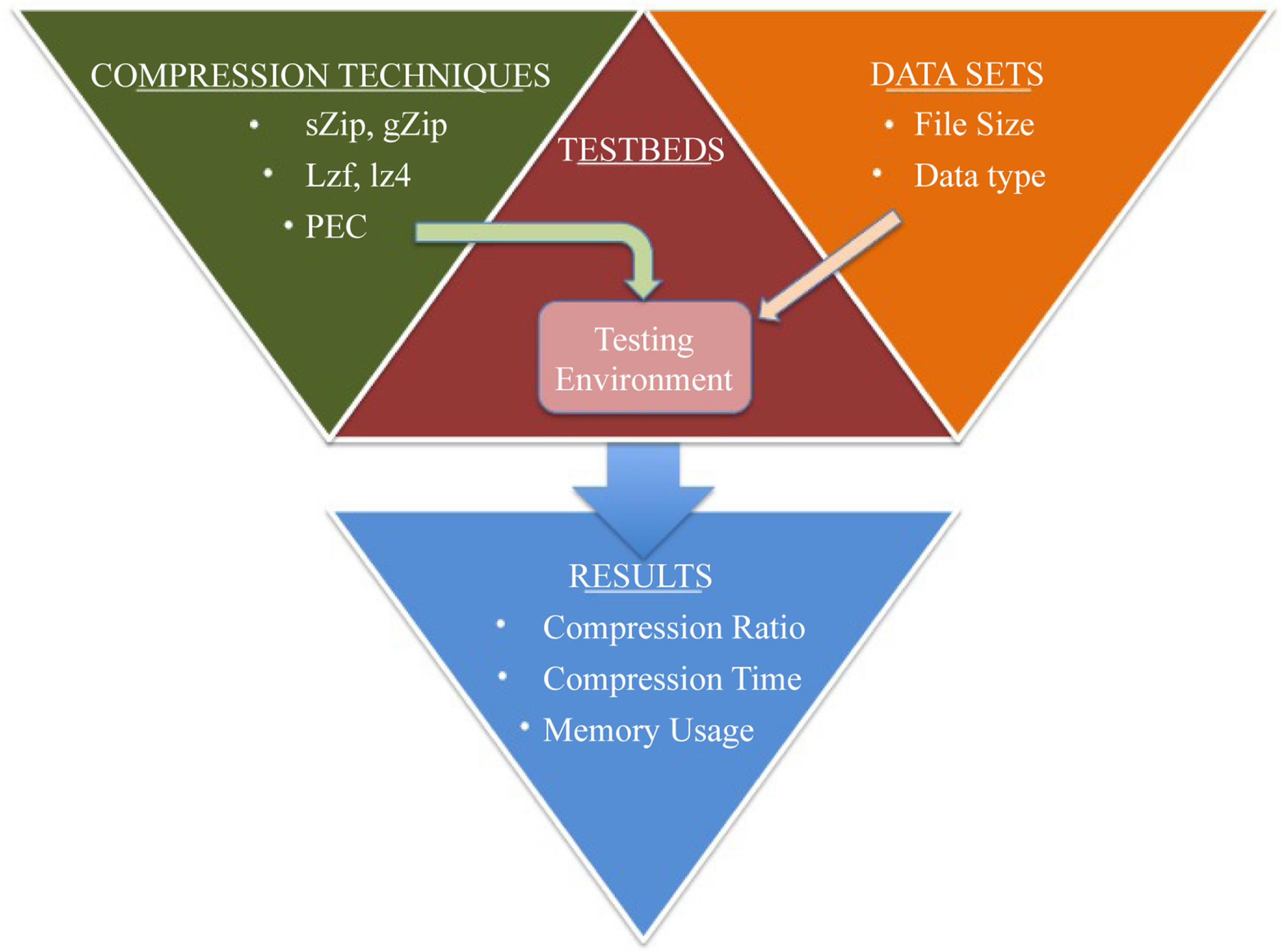
Figure 3. High level system design.
5.2. Datasets
A total of 11 datasets were obtained from the SKA. They ranged from 30 MB to 9.35 GB in size, of which 10 were collected during a 24 hour period on the 1st of December, 2012. File number 6 was collected on the 16th of December 2011. (Table 1) below shows each dataset and its size.
5.3. Compression Techniques
The selected lossless compression algorithms, SZIP, GZIP, LZF, FAPEC and LZ4, were installed and run on the primary testbed.
5.4. Streaming Compression
The aim of streaming compression is to compress a file while it is being read. This normally involves loading the file that is being read into memory and then applying the compression algorithm to the file. The effectiveness of this process relies heavily on the amount of RAM that is available and the size of the file that is being compressed.
Given the requirements for the project, two important factors had to be considered:
• The amount of time taken to compress the data while streaming;
• The time taken to send the file (network throughput).
These two metrics are crucial to the process of streaming compression as the trade-off between the time taken to compress the file and the time taken to send it would determine the effectiveness of streaming compression.
As a result, the following equations were established:
 (1)
(1)
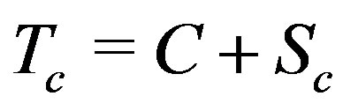 (2)
(2)
where:
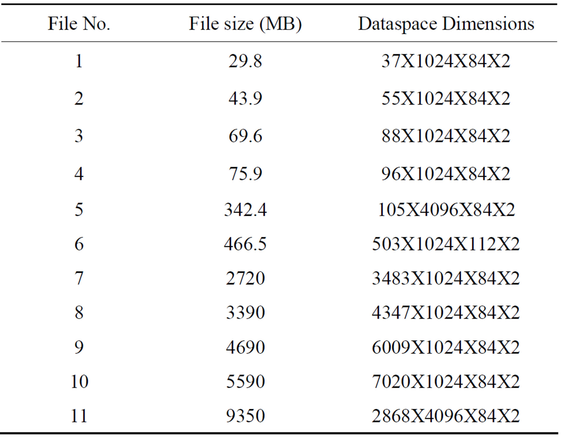
Table 1. List of the datasets.
• To is the total time taken to transfer the original file
• So is the time taken to stream the original file
• Tc is the total time taken to transfer the compressed file
• C is the time taken to the compress the file
• Sc is the time taken to stream the compressed file For streaming compression to be effective, Tsc would always have to be less than To.
5.4.1. SKA Compress
In order to explore the feasibility of streaming compression, a program was written which would perform the tasks shown in the following image. The program was named “SKA Compress”. The algorithm which was used to design the program is shown in (Figure 4).
The threshold of the file size would need to be set in the program depending on which compression algorithm was being used and the available network speed.
For example, if it took 30 seconds to transfer File A, and a total time of 40 seconds to compress and then transfer the compressed version of File A, the program would not compress the file and simply transfer. However, if it took 60 seconds to transfer a larger file (File B), and 50 seconds to compress and transfer the compressed version of File B, then the program would go ahead and compress the file and send it to the user.
The program was designed to take in the file that was to be opened as an input parameter. It would then compress the file, creating a compressed file named “tempfile”, which would then be sent to the user. Once the users have finished accessing the file, they could close the program, upon which the temporary file would be deleted.
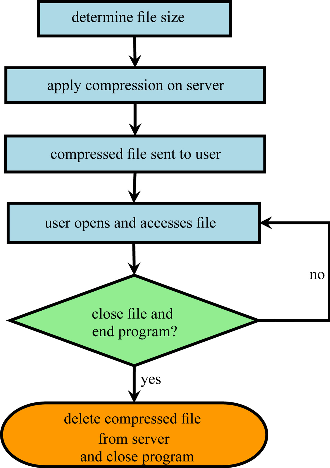
Figure 4. SKA compress flowchart.
Although the program would not strictly be compressing the file while it was being streamed to the user, the intention was for the program to operate so quickly that it would give the impression that stream-only compression was being achieved.
5.4.2. Stream-Only Compression
The final step was to implement stream-only compression i.e. applying the compression only while the file was being streamed from the primary testbed to the secondary testbed, neither before nor after.
The LZ4 algorithm implemented a function to carry out such a process, which was modified slightly to improve its performance. However, it was not tailored to suit the specific content and format of the files. Thus, it carried out a more generic approach towards the streamonly compression.
6. Results and Evaluation
Three phases of testing that were carried out, which were:
1) Initial performance testing 2) Final performance testing 3) Streaming compression testing
6.1. Initial Performance Testing
An inital set of testing was carried out smaller data sets to compare the performances of the different algorithms. These were files 1-6, which ranged from 29 MB to 466.5 MB in size.
This testing helped to give an indication of the algorithms’ compatibility with the specific arrangement and structure of these files, so that the best performing algorithms could be tested on the larger files (Figure 5).
The compression ratios, with the odd exception, gradually decreased as the file sizes increased, which is to be expected [18]. SZIP and GZIP provided the highest ratios, ranging between 1.4 - 1.6, while the FAPEC and LZ4 provided lower but consistent ratios. The LZF filter provided the lowest ratios. The relative compression ratios for SZIP, GZIP and LZF were in line with those that were found in the studies conducted by Yeh et al. [16] and Collette [17]. This was reflected further in the compression times.
The FAPEC and LZ4 were significantly faster than the other three algorithms. The LZ4 filter was also relatively quick while SZIP took longer, with GZIP being by far the slowest (Figure 6).
6.2. Final Performance Testing
The best three compression algorithms were selected from the initial testing in this stage. Based on the three key metrics, it was intended that the algorithms which
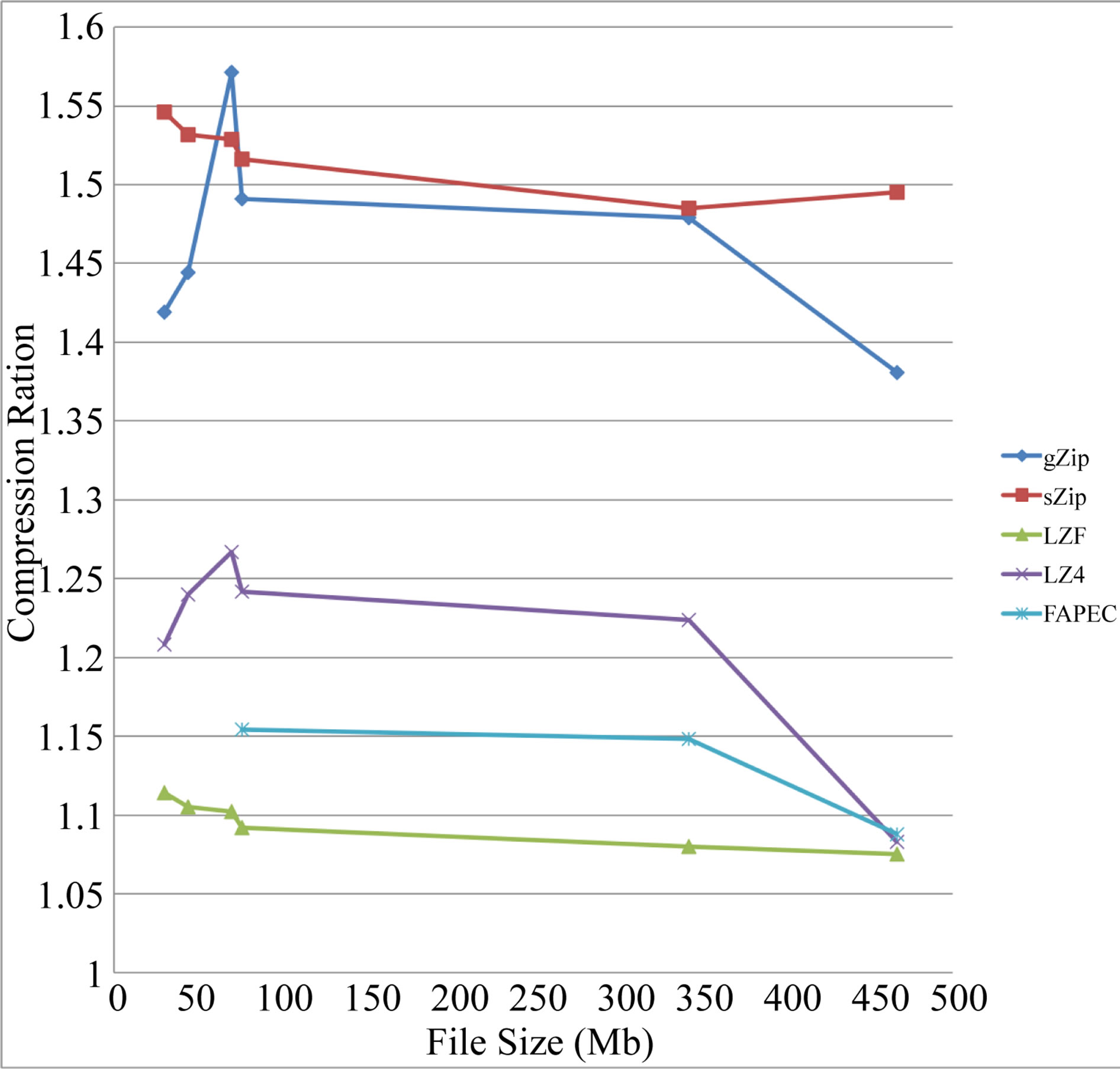
Figure 5. Compression ratios for initial performance testing.
provided the best ratio, quickest compression times and had the least memory usage would be selected. However, LZ4 provided the quickest compression speeds as well as the least memory usage, thus the FAPEC was chosen, as its ratio and timing results were very similar to those of LZ4. The final algorithm that was selected was SZIP, which provided the highest compression ratios.
Datsets 7-11 were used for LZ4 and SZIP, but only 7 and 8 could be used for the FAPEC due to time restrictions in sending the datasets to the researchers at the University of Barcelona.
Figure 7 below compares the compression ratios obtained from the final performance testing. As was with the inital stage, the FAPEC and LZ4 provided steady and similar ratios, ranging between 1.15 and 1.25. SZIP initially provided high ratios close to 1.5 for files 7 and 8, but its performance drastically declined on the three files greater than 4GB in size, reaching a similar level to that of LZ4.
Figure 8 compares the compression times obtained from the final performance testing. SZIP was considerably slower than the FAPEC and LZ4. In the most extreme case SZIP took almost 34 minutes longer than LZ4 to compress dataset 11. LZ4 was extremely quick, with the FAPEC performing slightly slower.
The results from this section clearly showed that LZ4 provided the best overall performances for the given data sets. It performed considerably faster than the other two algorithms, as well as being memory efficient and providing ratios greater than 1.1. As a result, it was chosen as the optimal algorithm to develop the stream-based system. The FAPEC provided promising results which were likely to be close to those achieved by LZ4.
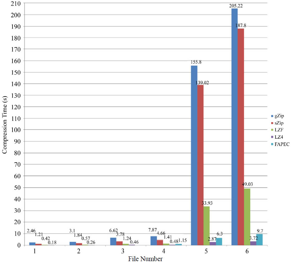
Figure 6. Compression times for initial performance testing.
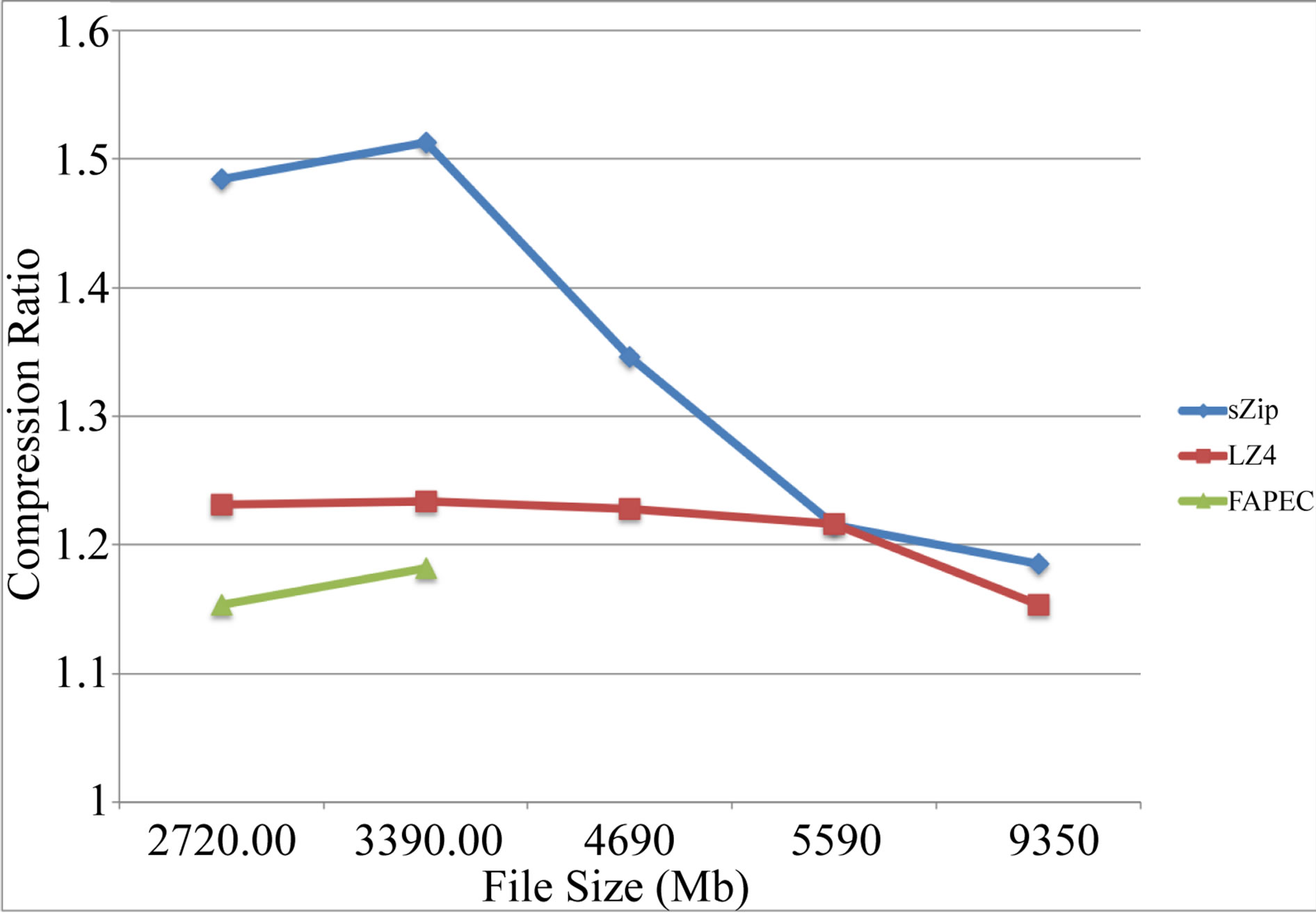
Figure 7. Compression ratios for final performance testing.
6.3. Streaming Compression Testing
The results in this section are split into two sub-sections, those from the initial stage of the SKA Compress program, and those when stream-only compression was integrated and attempted.
SKA Compress
The transfer speed from the server testbed to the main testbed averaged between 2.5 MB/s and 2.8 MB/s.
Figures 9 and 10 show the time taken to transfer the original, uncompressed files and the compressed files. The first graph shows the results for datasets 1-6, and the second graph shows the results from datasets 7- 11.
Using Equations (1) and (2), for streaming compression to be effective, Tc needed to be less than To. The two graphs show that Tc was less than To for all of the datasets except number 6, where a lower compression ratio of 1.083 was obtained. The difference in time between To and Tc increased as the files got larger in size, while the difference was small (less than 5 seconds on average) with files smaller than 100 MB.
This showed that SKA Compress performed successfully and met the objective of providing results where Tc was consistently less than To.
6.4. Stream-Only Compression
The final step was to implement stream-only compression i.e. applying the compression only while the file was being streamed from the server testbed to the main testbed, neither before nor after.
Figures 11 and 12 show the results that were obtained from stream-only compression.
As shown in Figure 12, the time taken to compress and stream the files generally took much longer than it
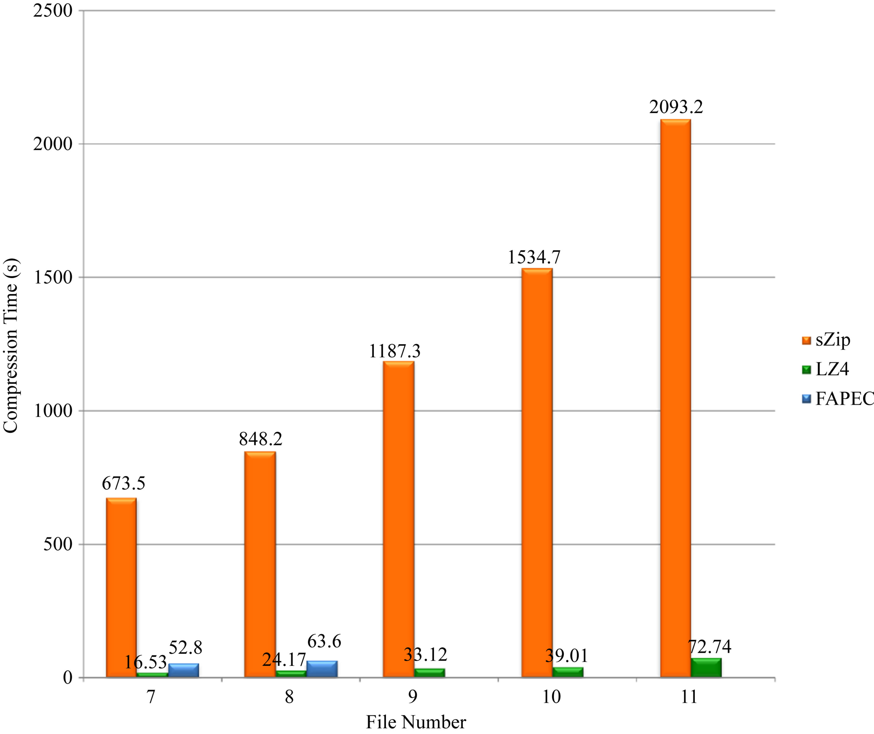
Figure 8. Compression times for final performance testing.
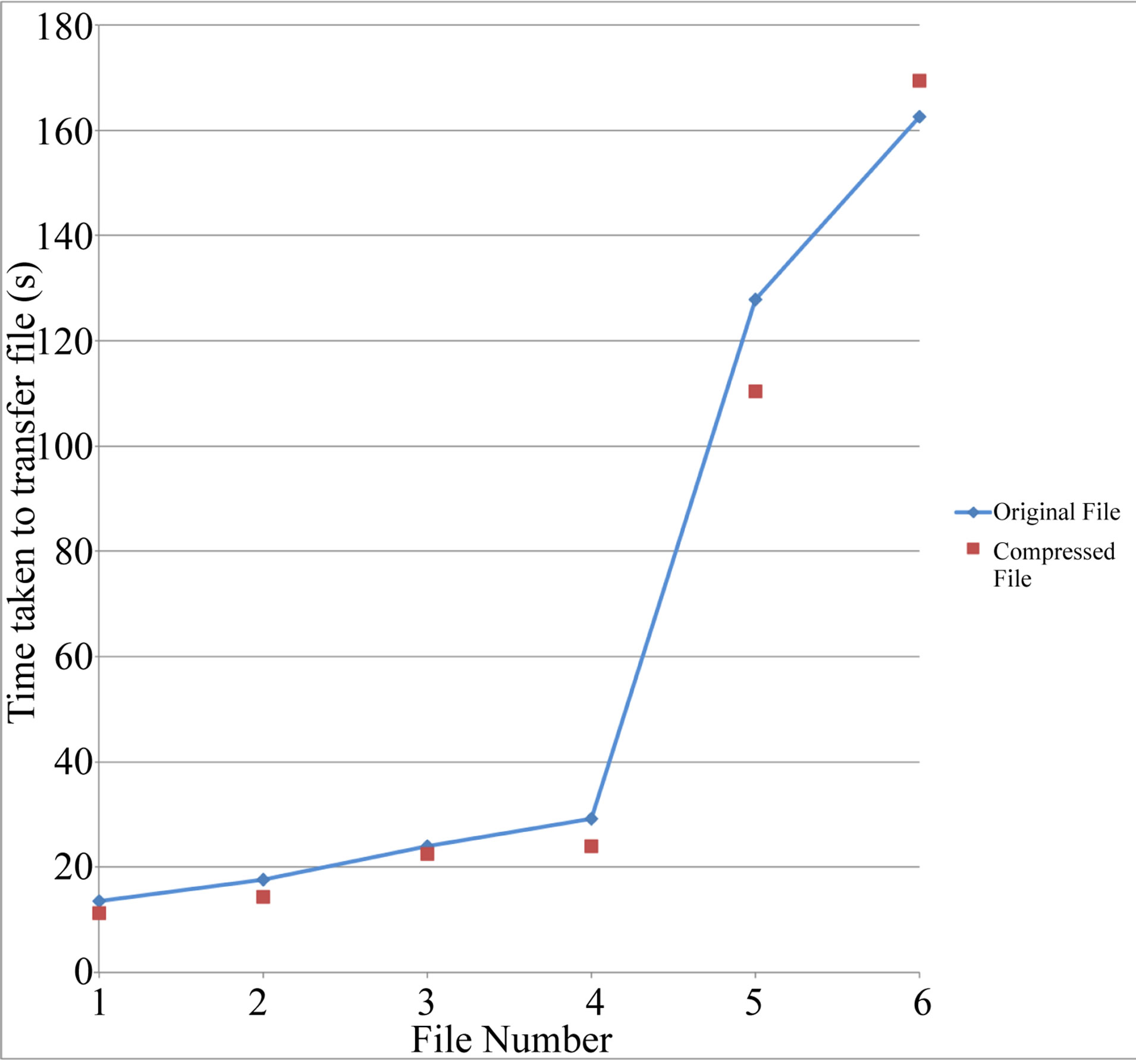
Figure 9. Comparing the streaming compression times for datasets 1-6.
would to simply transfer the original, uncompressed files. The stream-only compression program performed in a time efficient manner for the first three files. For every file after that, the differences in the time taken were progressively longer. The one outlier result for SKA Compress was due to the file becoming corrupted during that
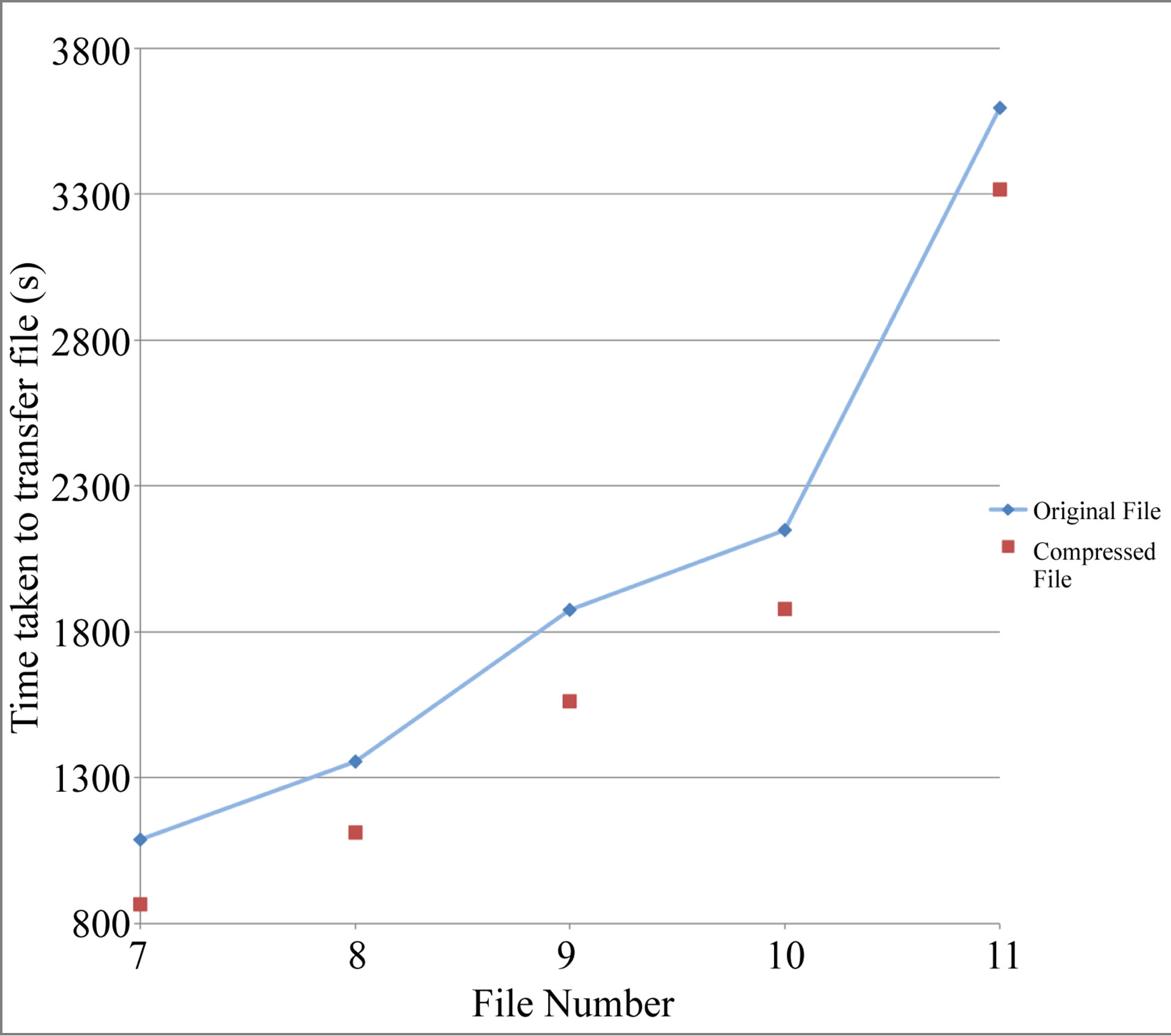
Figure 10. Comparing the streaming compression times for datasets 7-11.
set of testing.
The compression ratios obtained through stream-only compression were comparable to those from SKA Compress for the first four files. However, there was a drastic decrease for every file after that. The compression ratio dropped to a very low level, such that the ratio obtained for file 11 was entirely negligible, with the compressed
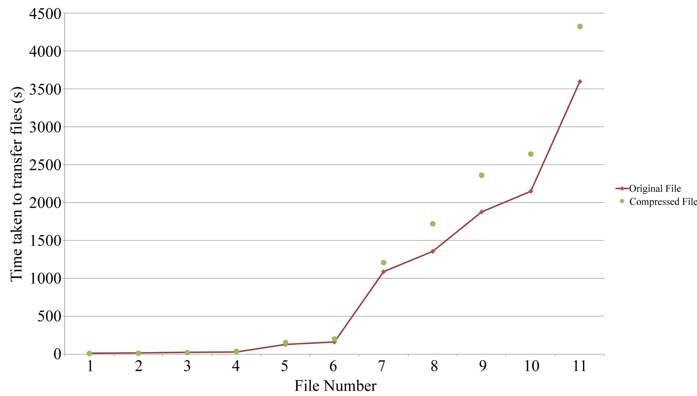
Figure 11. Comparing the compression times between To and Sc.
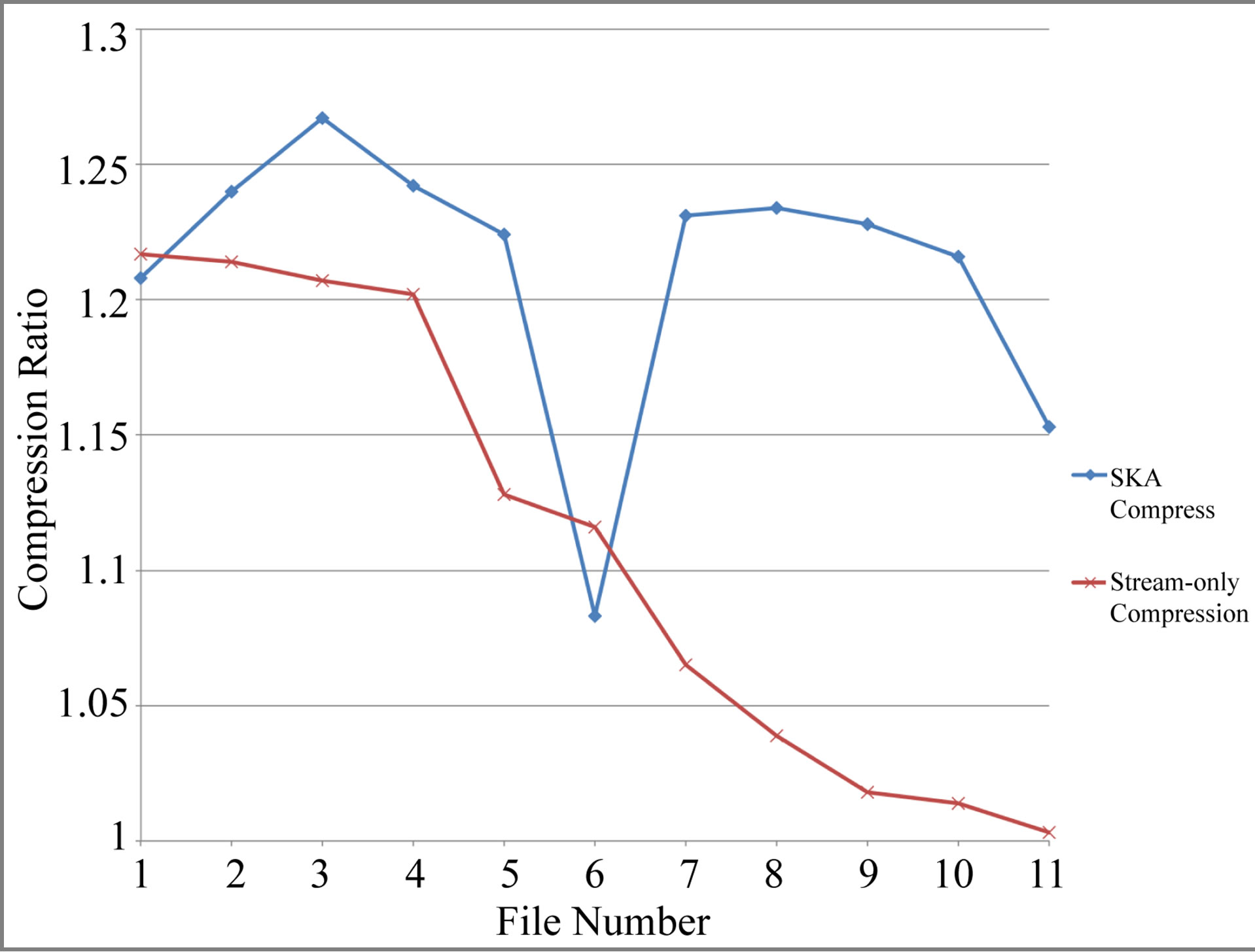
Figure 12. Comparing the compression ratios between SKA Compress and stream-only compression.
file only 0.03% smaller than the original. This can be attributed to the larger block sizes that had to be sent through the memory buffer.
One of the problems that came up from stream-only compression was that the compressed versions of files 7- 11 could not be read and were corrupted. Given that file 7 is 2.7 GB in size, it was suspected that the reason for those outcomes was a result of the header of the files and the end of the files not reaching the user in the same session. It was observed that when memory usage became extremely high (greater than 50%), the disk would be in a “sleeping” state and thus the process would be paused for a short period time, before resuming. In that period, it is likely that the files greater in size than half of the available RAM (which would be 1 GB) caused the disk to enter the ‘sleeping’ state, thus not concatenating the header with the end of the file.
As a result, although the entire compressed files would reach the user, they were not in the exact same format and structure as the original, causing them to be corrupted.
7. Conclusions and Recommendations
The FAPEC and LZ4 provided the best overall results, and both algorithms achieved this while being significantly faster and using less memory than the other three. The commercial restrictions of the FAPEC did not allow for more rigorous testing. However, the nature of the algorithm and the results it provided were very promising. The LZ4 results provided the best performance when considering the key performance metrics and they were successfully used to develop the SKA Compress program.
The results using SKA Compress were excellent and met most of the criteria detailed in the requirements for the project. They showed that it was possible to run a program which eased the load on the available computing resources (storage space and memory) and allowed users to access the datasets in a time efficient manner. It was also evident that certain thresholds would need to be set within the program based on the network speed, in order to maximize its performance.
The outcome of attempting stream-only compression was not entirely successful, as it was extremely memory intensive and regularly created corrupted datasets which could not be read by the end user. However, the few successful attempts indicate that it is an aspect which needs to be worked on and could provide hugely beneficial outcomes if improved upon.
The following lists of recommendations are intended to provide a guideline to build upon the work carried out in this study.
1) Test on greater number of datasets—While this study managed to cover a wide range of datasets, more accurate results could be obtained by testing a greater number of files within the same range. This would provide clearer indications on how to optimize parameters in the compression programs, particularly with regard to pure streaming compression.
2) Refinement of LZ4 to be more specific to the datasets—The LZ4 algorithm provided excellent results in all three key metrics. However, the algorithm was only slightly modified and was run without considering the format or contents of the files. Tailoring the performance of the LZ4 algorithm to the HDF5 format and treating dataspaces within the datasets based on the nature of the data, could yield much better results.
3) Obtain final version of FAPEC—The FAPEC provided very similar results to LZ4, but it was slightly slower. However, the nature of the FAPEC means that it is designed to progressively compress the HDF5 files as they are being transferred/streamed, and that it is fully adaptive. This would indicate that the final commercial version of the FAPEC could provide even better and more specifically applicable compression.
8. Acknowledgements
We acknowledge the intellectual contributions of our colleagues in the Radar and Remote Sensing Group at the University of Cape Town. This research was done in collaboration with the South African SKA MeerKAT project.
REFERENCES
- L.-L. Stark and F. Murtagh, “Handbook of Astronomical Data Analysis,” Springer-Verlag, Heidelberg-Berlin, 2002.
- W. D. Pence, R. Seaman and R. L. White, “Lossless Astronomical Image Compression and the Effects of Noise,” Publications of the Astronomical Society of the Pacific, Vol. 121, No. 4, 2009, pp. 414-427. http://dx.doi.org/10.1086/599023
- “South Africa’s Meerkat Array,” 2012. http://www.ska.ac.za/download/factsheetmeerkat2011.pdf
- R. Mittra, “Square Kilometer Array-A Unique Instrument for Exploring the Mysteries of the Universe Using the Square Kilometer Array,” Applied Electromagnetics Conference (AEMC), Kolkata, 14-16 December 2009, pp. 1-6.
- D. L. Jones, K. Wagstaff, D. R. Thompson, L. D’Addario, R. Navarro, C. Mattmann, W. Majid, J. Lazio, R. Preston, and U. Rebbapragada, “Big Data Challenges for Large Radio Arrays,” IEEE Aerospace Conference, Big Sky, 3-10 March 2012, pp. 1-6.
- J.-L. Starck and F. Murtagh, “Astronomical Image and Signal Processing,” IEEE Signal Processing Magazine, Vol. 18, No. 2, 2002, pp. 30-40.
- S. de Rooij and P. M. Vitanyi, “Approximating Rate-Distortion Graphs of Individual Data: Experiments in Lossy Compression and Denoising,” IEEE Transactions on Computers, Vol. 23, No. 4, 2012, pp. 14-15.
- S. Finniss, “Using the Fits Data Structure,” Master’s Thesis, University of Cape Town, Cape Town, 2011.
- K. Borne, “Data Science Challenges from Distributed Petascale Astronomical Sky Surveys,” DOE Conference on Mathematical Analysis of Petascale Data, 2008.
- K. R. Anderson, A. Alexov, L. BaŁhren, J. M. Griemeier, M. Wise, and G. A. Renting, “LOFAR and HDF5: Toward a New Radio Data Standard,” SKAF2010 Science Meeting, 10-14 June 2010.
- B. B. C. I. of Technology, “Astronomy Needs New Data Format Standards,” 2011. http://astrocompute.wordpress.com/2011/05/20/astronomy-needs-new-data-format-standards/
- “Hdf5 for Python,” 2013. www.alvfen.org/wp/hdf-5for-python
- C. E. Sanchez, “Feasibility Study of the PEC Compressor in hdf5 File Format,” Master’s Thesis, Universitat Politecnica de Catalunya, 2011.
- “What Is HDF5,” 2013. www.hdfgroup.org/hdf5/whatishdf5.html
- P.-S. Yeh, W. Xia-Serafino, L. Miles, B. Kobler and D. Menasce, “Implementation of CCSDS Lossless Data Compression in HDF,” Space Operations Conference, Houston, 9-12 October 2002.
- “Implementation of CCSDS Lossless Data Compression in HDF,” Earth Science Technology Conference, Pasadena, 11-13 June 2002.
- “LZF Compression Filter for HDF5,” 2013. http://www.h5py.org/lzf/
- J. Portell, E. Garcia Berroad, C. E. Sanchez, J. Castaneda, and M. Clotet, “Efficient Data Storage of Astronomical Data Using HDF5 and PEC Compression,” SPIE HighPerformance Computing in Remote Sensing, Vol. 8183, 2011, Article ID: 818305.
- “LZ4 Explained,” 2013. http://fastcompression.blogspot.com/2011/05/lz4-explained.html
- “From Big Bang to Big Data: Astron and IBM Collaborate to Explore Origins of the Universe,” 2012. http://www-03.ibm.com/press/us/en/pressrelease/37361.wss