Advances in Pure Mathematics
Vol.2 No.6(2012), Article ID:24971,13 pages DOI:10.4236/apm.2012.26065
Construction of Zero Autocorrelation Stochastic Waveforms*
Department of Mathematics, University of Idaho, Moscow, USA
Email: sdatta@uidaho.edu
Received July 18, 2012; revised September 10, 2012; accepted September 17, 2012
Keywords: Autocorrelation; Frames; Stochastic Waveforms
ABSTRACT
Stochastic waveforms are constructed whose expected autocorrelation can be made arbitrarily small outside the origin. These waveforms are unimodular and complex-valued. Waveforms with such spike like autocorrelation are desirable in waveform design and are particularly useful in areas of radar and communications. Both discrete and continuous waveforms with low expected autocorrelation are constructed. Further, in the discrete case, frames for  are constructed from these waveforms and the frame properties of such frames are studied.
1. Introduction
1.1. Motivation
Designing unimodular waveforms with an impulse-like autocorrelation is central in the general area of waveform design, and it is particularly relevant in several applications in the areas of radar and communications. In the former, the waveforms can play a role in effective target recognition, e.g., [1-8]; and in the latter they are used to address synchronization issues in cellular (phone) access technologies, especially code division multiple access (CDMA), e.g., [9,10]. The radar and communications methods combine in recent advanced multifunction RF systems (AMRFS). In radar there are two main reasons that the waveforms should be unimodular, that is, have constant amplitude. First, a transmitter can operate at peak power if the signal has constant peak amplitude—the system does not have to deal with the surprise of greater than expected amplitudes. Second, amplitude variations during transmission due to additive noise can be theoretically eliminated. The zero autocorrelation property ensures minimum interference between signals sharing the same channel.
Constructing unimodular waveforms with zero autocorrelation can be related to fundamental questions in harmonic analysis as follows. Let  be the real numbers,
  the integers,
  the complex numbers, and set
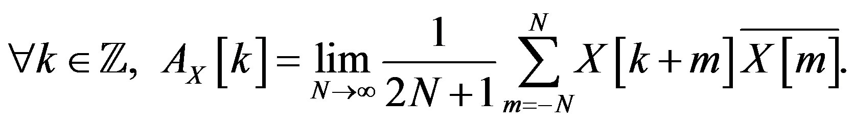
 . The aperiodic autocorrelation
  of a waveform
 , is defined as
 (1)
(1)
A general problem is to characterize the family of positive bounded Radon measures F, whose inverse Fourier transforms are the autocorrelations of bounded waveforms X. A special case is when  on
on  and X is unimodular on
 . This is the same as when the autocorrelation of X vanishes except at 0, where it takes the value 1. In this case, X is said to have perfect autocorrelation. An extensive discussion on the construction of different classes of deterministic waveforms with perfect autocorrelation can be found in [11]. Instead of aperiodic waveforms that are defined on
 , in some applications, it might be useful to construct periodic waveforms with similar vanishing properties of the autocorrelation function. Let
  be an integer and
  be the finite group
  with addition modulo n. The periodic autocorrelation
 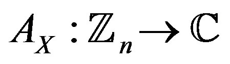 of a waveform
  is defined as
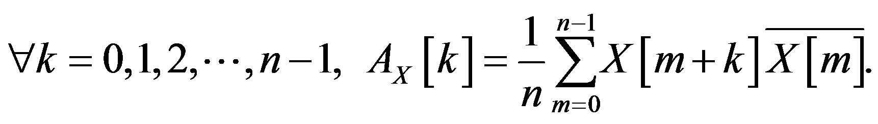 (2)
(2)
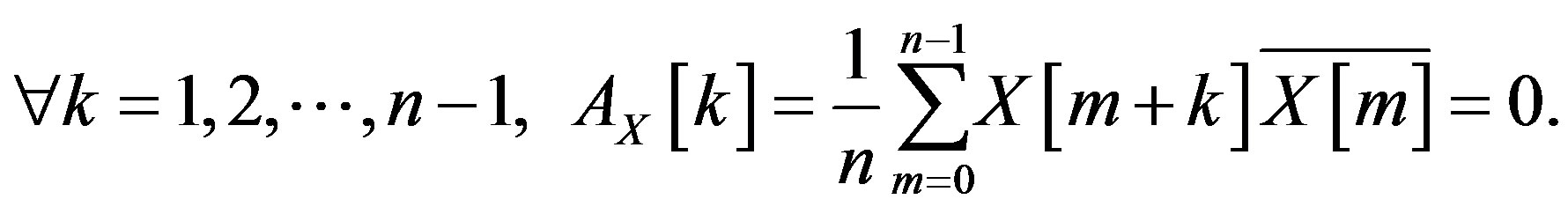
It is said that  is a constant amplitude zero autocorrelation (CAZAC) waveform if each
  and
and
The literature on CAZACs is overwhelming. A good reference on this topic is [3], among many others. Literature on the general area of waveform design include [12-14]. Comparison between periodic and aperiodic autocorrelation can be found in [15].
Here the focus is on the construction of stochastic aperiodic waveforms. Henceforth, the reference to waveforms shall imply aperiodic waveforms unless stated otherwise. These waveforms are stochastic in nature and are constructed from certain random variables. Due to the stochastic nature of the construction, the expected value of the corresponding autocorrelation function is analyzed. It is desired that everywhere away from zero, the expectation of the autocorrelation can be made arbitrarily small. Such waveforms will be said to have almost perfect autocorrelation and will be called zero autocorrelation stochastic waveforms. First discrete waveforms,  , are constructed such that X has almost perfect autocorrelation and for all
 This approach is extended to the construction of continuous waveforms,
  , with similar spike like behavior of the expected autocorrelation and
  for all
  Thus, these waveforms are unimodular. The stochastic and non-repetitive nature of these waveforms means that they cannot be easily intercepted or detected by an adversary. Previous work on the use of stochastic waveforms in radar can be found in [16-18], where the waveforms are only real-valued and not unimodular. In comparison, the waveforms constructed here are complex valued and unimodular. In addition, frame properties of frames constructed from these stochastic waveforms are discussed. This is motivated by the fact that frames have become a standard tool in signal processing. Previously, a mathematical characterization of CAZACs in terms of finite unit-normed tight frames (FUNTFs) has been done in [2].
1.2. Notation and Mathematical Background
Let  be a random variable with probability density function
  Assuming
  to be absolutely continuous, the expectation of
  denoted by
  is
is
The Gaussian random variable has probability density function given by  The mean or expectation of this random variable is
  and the variance,
  is
is  In this case it is also said that
  follows a normal distribution and is written as
  The characteristic function of
  at
at 
 , is denoted by
 . For further properties of expectation and characteristic function of a random variable the reader is referred to [19].
Let  be a Hilbert space and let
  where
where  is some index set, be a collection of vectors in
 . Then
  is said to be a frame for
  if there exist constants
  and
and 
 such that for any
The constants A and B are called the frame bounds. Thus a frame can be thought of as a redundant basis. In fact, for a finite dimensional vector space, a frame is the same as a spanning set. If  the frame is said to be tight. Orthonormal bases are special cases of tight frames and for these,
If  is a frame for
  then the map
  given by
  is called the analysis operator. The synthesis operator is the adjoint map
  given by
The frame operator  is given by
  For a tight frame, the frame operator is just a constant multiple of the identity, i.e.,
  where
where  is the identity map. Every
  can be represented as
Here  is also a frame and is called the dual frame. For a tight frame,
  is just
  Tight frames are thus highly desirable since they offer a computationally simple reconstruction formula that does not involve inverting the frame operator. The minimum and maximum eigenvalues of
  are the optimal lower and upper frame bounds respectively [20]. Thus, for a tight frame all the eigenvalues of the frame operator are equal to each other. For the general theory on frames one can refer to [20,21].
1.3. Outline
The construction of discrete unimodular stochastic waveforms,  , with almost perfect autocorrelation is done in Section 2. This is first done with the Gaussian random variable and then generalized to other random variables. The variance of the autocorrelation is also estimated. The section also addresses the construction of stochastic waveforms in higher dimensions, i.e., construction of
 , that have almost perfect autocorrelation and are unit-normed, considering the usual norm in
  In Section 3 the construction of unimodular continuous waveforms with almost perfect autocorrelation is done using Brownian motion.
As mentioned in Section 1.2, frames are now a standard tool in signal processing due to their effectiveness in robust signal transmission and reconstruction. In Section 4, frames in  are constructed from the discrete waveforms of Section 2 and the nature of these frames is analyzed. In particular, the maximum and minimum eigenvalues of the frame operator are estimated. This helps one to understand how close these frames are to being tight. Besides, it follows, from the eigenvalue estimates, that the matrix of the analysis operator, F, for such frames, can be used as a sensing matrix in compressed sensing.
2. Construction of Discrete Stochastic Waveforms
In this section discrete unimodular waveforms,  , are constructed from random variables such that the expectation of the autocorrelation can be made arbitrarily small everywhere except at the origin. First, such a construction is done using the Gaussian random variable. Next, a general characterization of all random variables that can be used for the purpose is given.
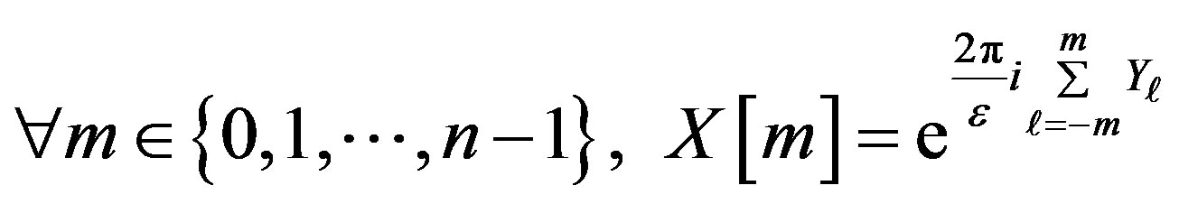
2.1. Construction from Gaussian Random Variables
Let  be independent identically distributed (i.i.d.)
random variables following a Gaussian or normal distribution with mean 0 and variance  i.e.,
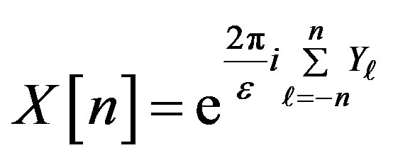
i.e.,  Define
  by
by
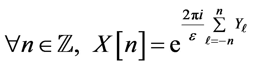 (3)
(3)
where i is . Thus, for each
 ,
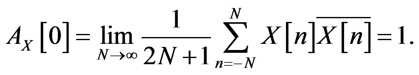
,  and X is unimodular. The autocorrelation of X at
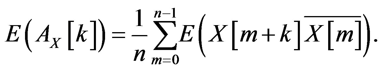
  is
is
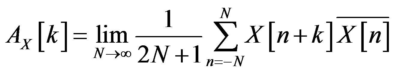
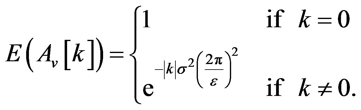
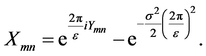
where the limit is in the sense of probability. Theorem 2.1 shows that the waveform given by (3) has autocorrelation whose expectation can be made arbitrarily small for all integers 
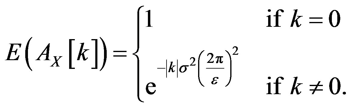
Theorem 2.1. Given  the waveform
  defined in (3) has autocorrelation
  such that
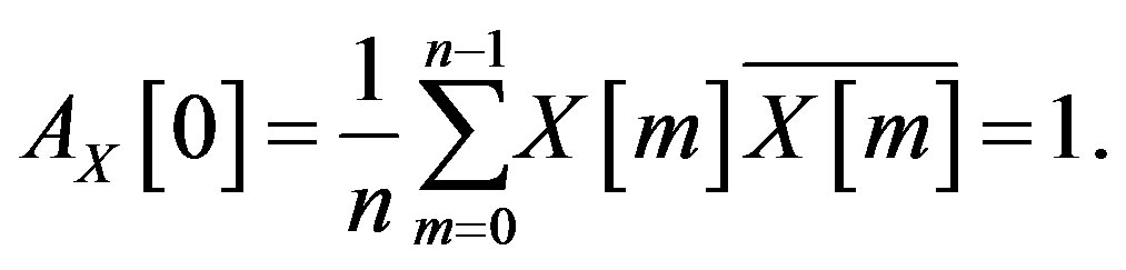
Proof. 1) When 
and so 
2) Let  One would like to calculate
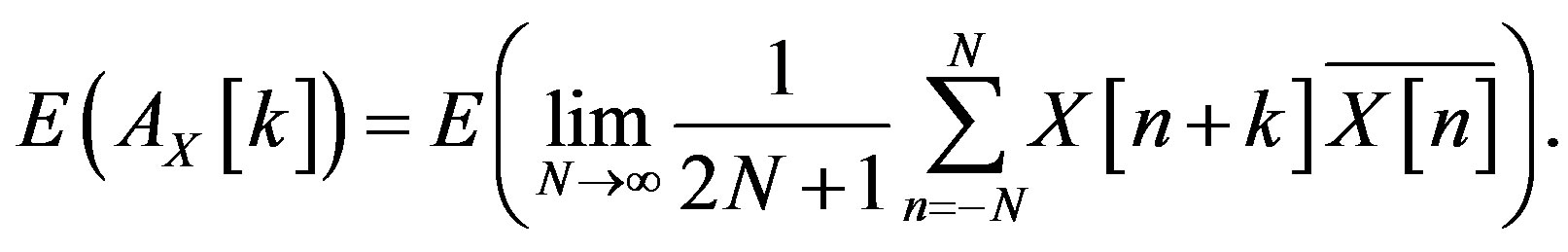
Let 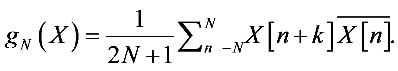 Then
Then  Let
Let  Then for each
 and
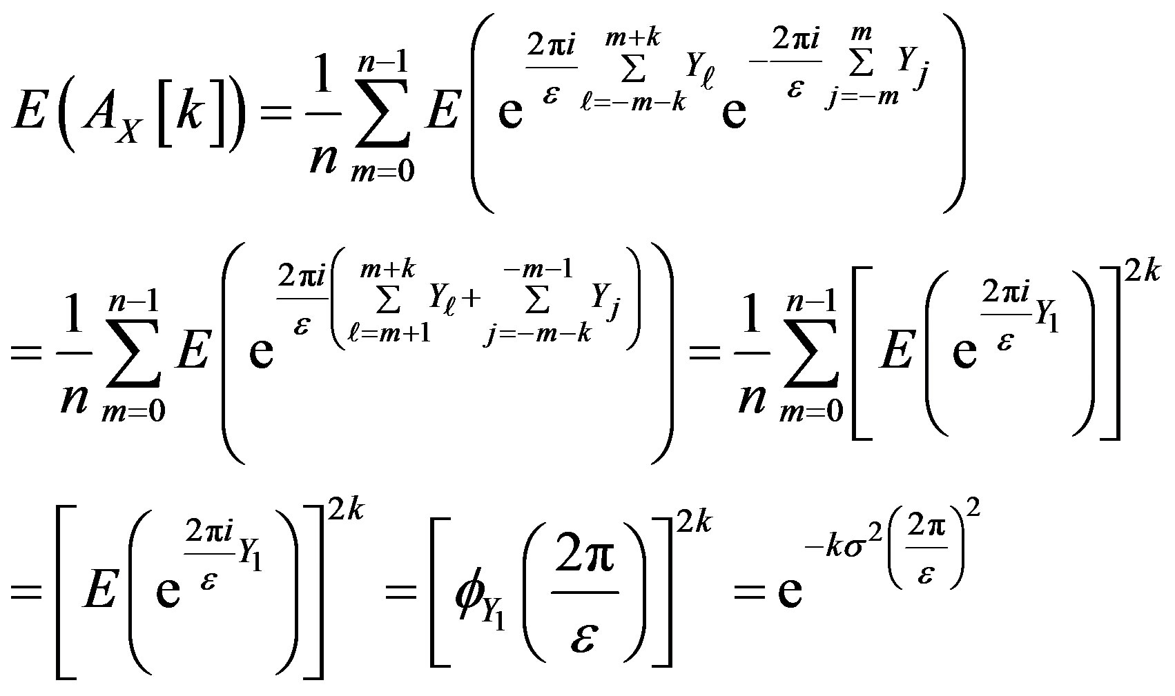
and . Thus, by the Dominated Convergence Theorem [19], which justifies the interchange of limit and integration below, one obtains
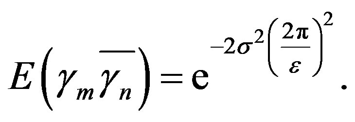
where the last line uses the fact that the  s are i.i.d. random variables. Here
  is the characteristic function at
  of
of  which is the same as that for any other
  due to their identical distribution. The characteristic function at
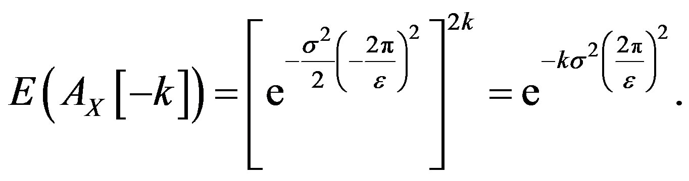
  of a Gaussian random variable with mean 0 and variance
  is
is  Thus
Thus
3) When  a similar calculation for
  gives
gives
Together, this shows that given  and any
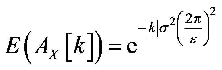
which indicates that the expectation of the autocorrelation at any integer  can be made arbitrarily small depending on the choice of
 . □
. □
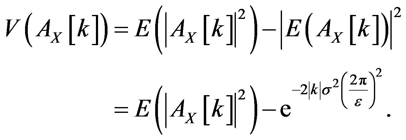
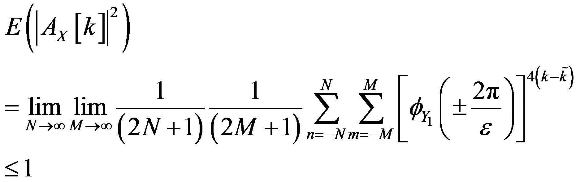
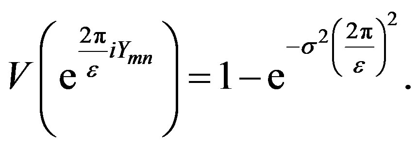
As shown in Theorem 2.1 the expectation of the autocorrelation can be made arbitrarily small but this is not useful unless one can estimate the variance of the autocorrelation. Denoting the variance of  by
by
 one has
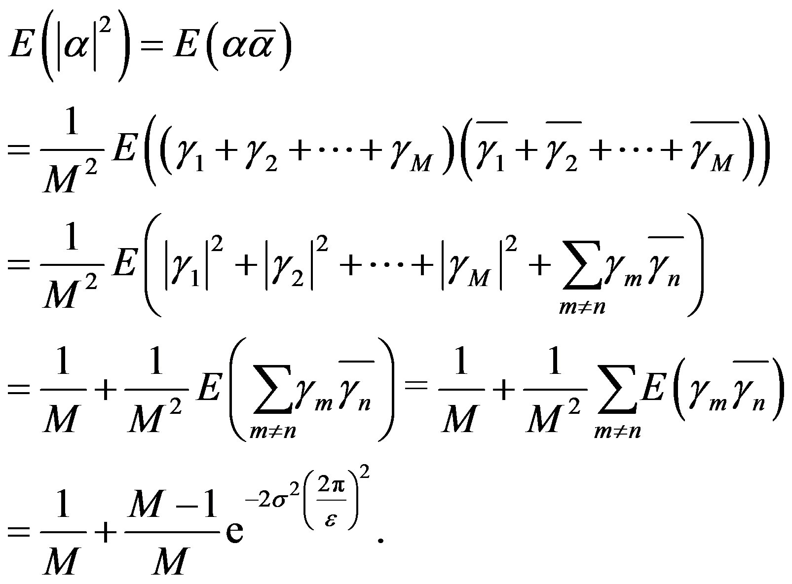
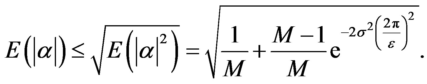
First consider 
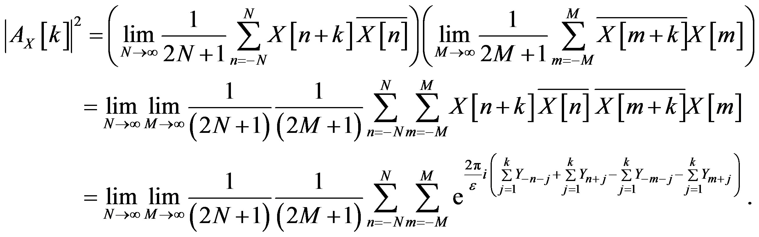
By applying the Lebesgue Dominated Convergence Theorem one can bring the expectation inside the double sum to get
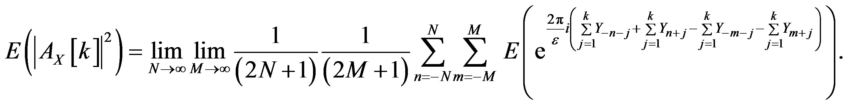
The sum
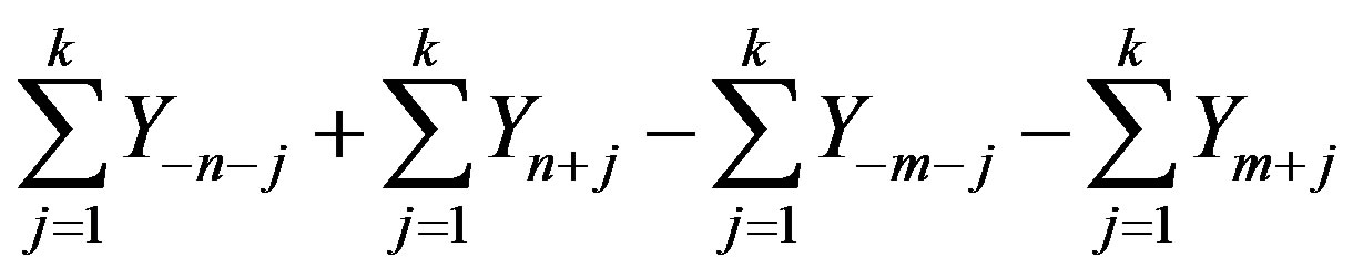 (4)
(4)
may have cancelations among terms involving n with terms involving m. Suppose that for a fixed n and m there are  indices that cancel in each of the four sums in (4). Due to symmetry, the same number i.e.,
  of terms will cancel in each sum. Depending on n and m,
  lies between 0 and k, i.e.,
  For the sake of making the notation less cumbersome,
  will from now on be written as
 . When
 If
If  or
or  then
then  Each sum in (4) has k terms and
  of these get cancelled leaving
  terms. One can re-index the variables in (4) and write it as
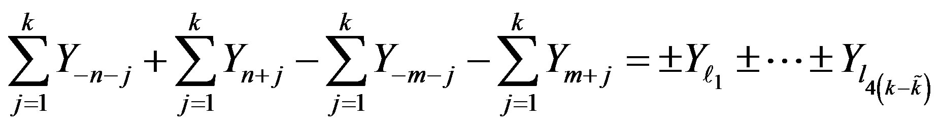
where the sign depends on whether  is less than or greater than
  Thus
Thus
 .
.
Due to the independence of the  s, this means
The minimum is attained for  and the maximum at
  Thus
Thus
and
This gives
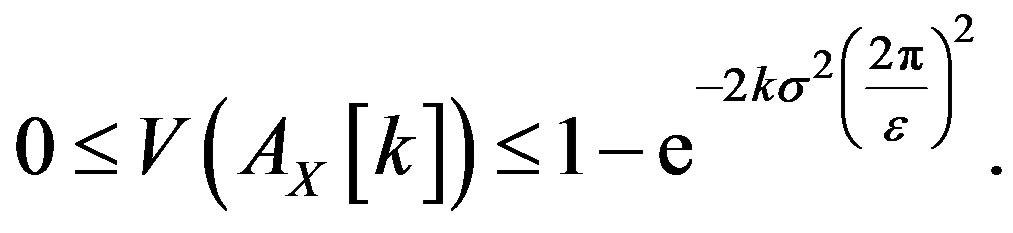
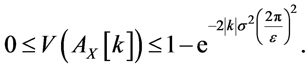
A similar calculation can be done for  Thus for
2.2. Generalizing the Construction to Other Random Variables
So far the construction of discrete unimodular zero autocorrelation stochastic waveforms has been based on Gaussian random variables. This construction can be generalized to many other random variables. The unimodularity of the waveforms is not affected by using a different random variable. The following theorem characterizes the class of random variables that can be used to get the desired autocorrelation.
Theorem 2.2. Let  be a sequence of i.i.d. random variables with characteristic function
  Suppose that the probability density function of the
  s is even and that
  goes to 0 as t goes to infinity. Then, given
  the waveform
  given by
has almost perfect autocorrelation.
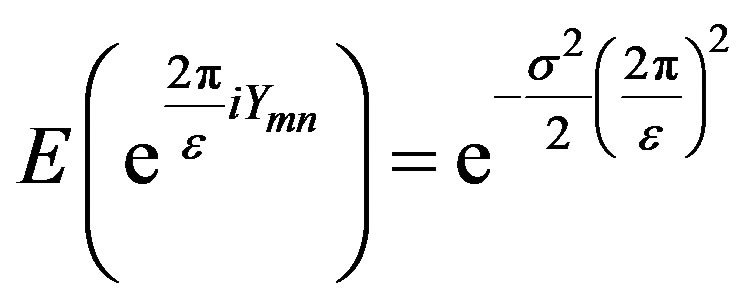
Proof. Since the density function of each  is even this means that the characteristic function is real valued [19]. Following the calculation in the proof of Theorem 2.1, the expected autocorrelation of
  for
for  is
is
and this goes to zero with  by the hypothesis. □
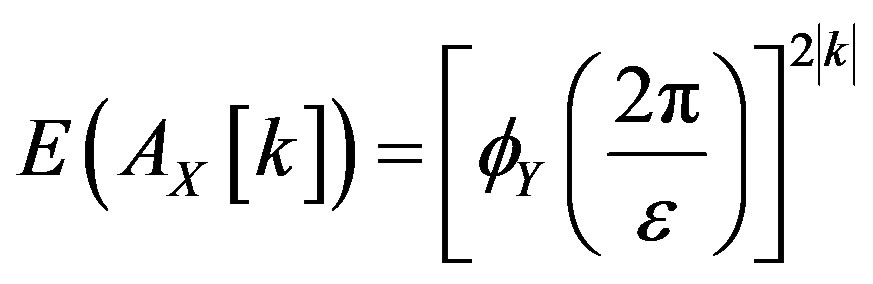
Example 2.3. Suppose the  s follow a bilateral distribution that has density
  with
with  and characteristic function
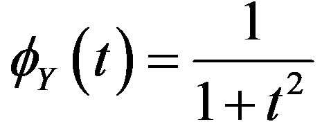 . Then for
 ,
,
and this can be made arbitrarily small with .
.
In the same way as was done in the Gaussian case, for 
and
Thus
Example 2.4. Suppose that the  s follow the Cauchy distribution with density function
  Note thatdisregarding the constant
  this is the characteristic function of the random variable considered in Example 2.3. The characteristic function of the
  s is now
  the same as the distribution function in Example 2.3. For
which can be made arbitrarily small with  Also,
Also,
2.3. Higher Dimensional Case
Here one is interested in constructing waveforms 
 ,
,  It is desired that
  has unit norm and the expectation of its autocorrelation can be made arbitrarily small. One way to construct
  is based on the construction of the one dimensional example given in Section 2.1. This is motivated by the higher dimensional construction in the deterministic case [2]. As before,
  is a sequence of i.i.d. Gaussian random variables with mean zero and variance
 . Next, one defines
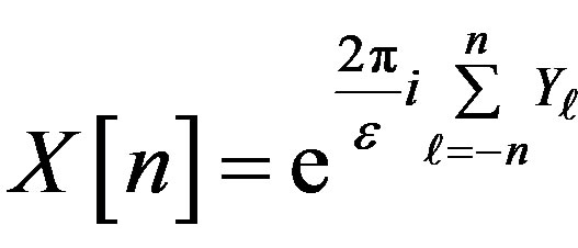 . The waveform
  is then defined as
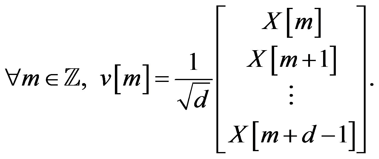 (5)
(5)
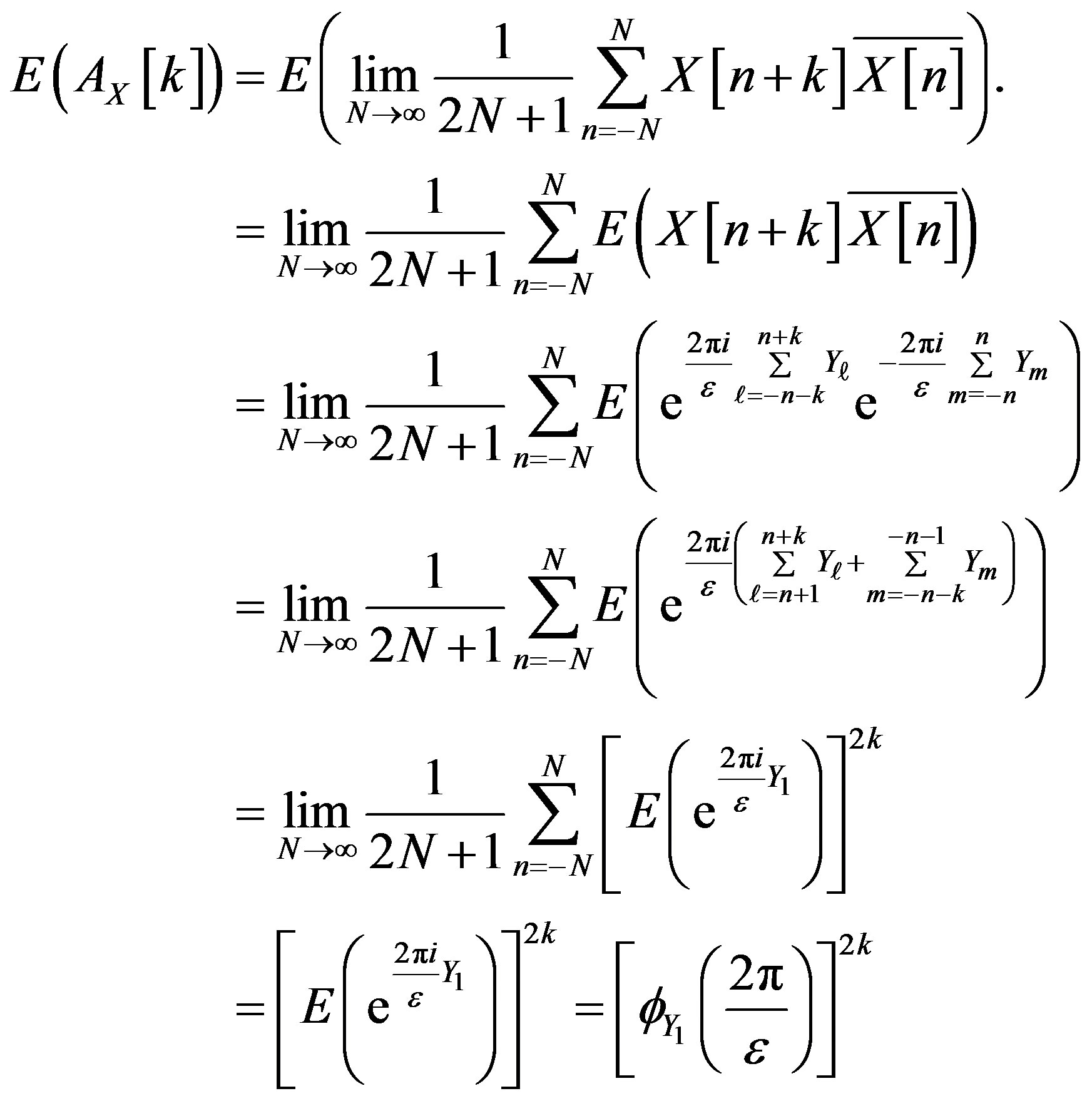
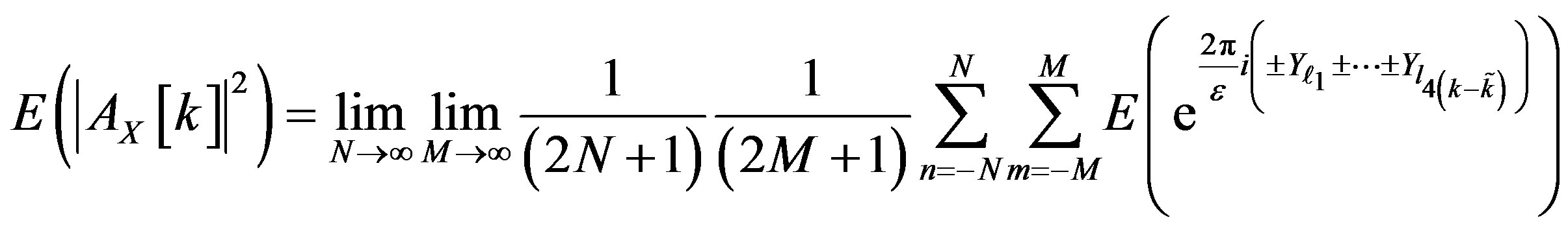
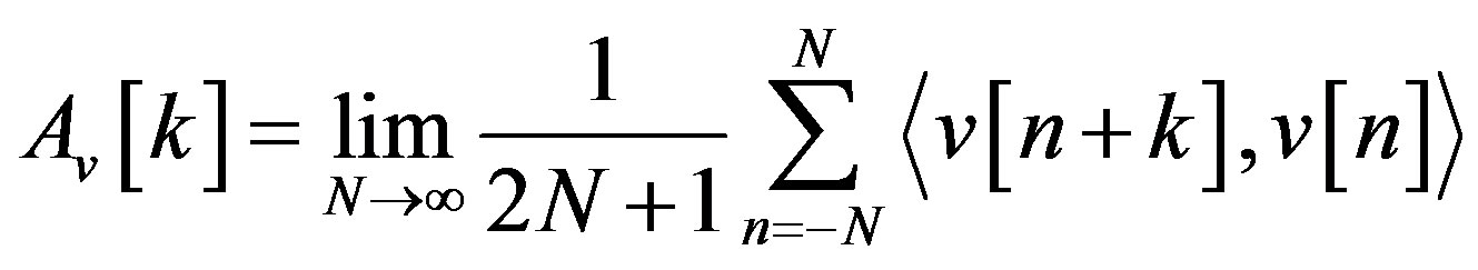
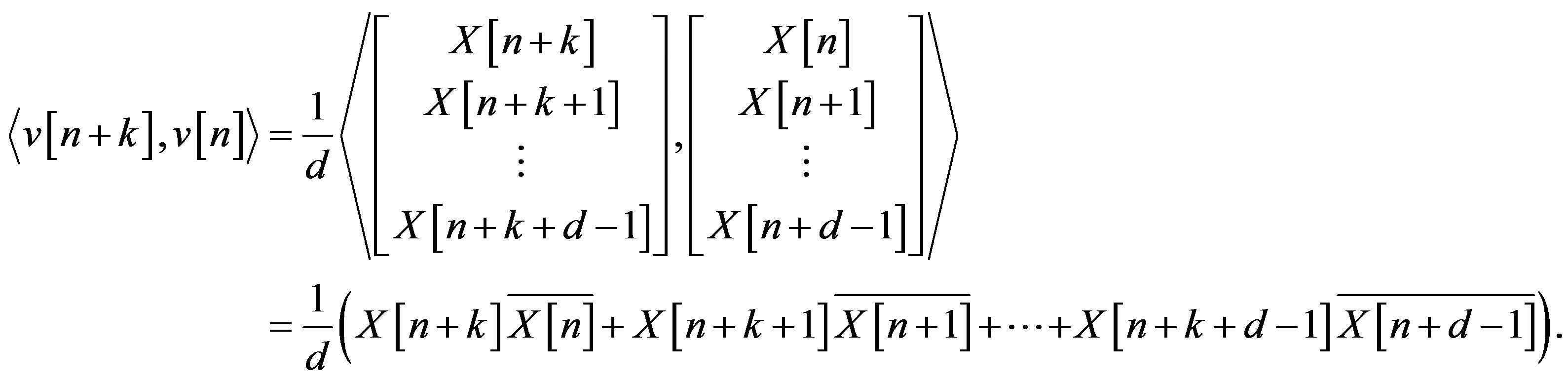
In this case, the autocorrelation is given by
 (6)
(6)
where  is the usual inner product in
 . The length or norm of any
  is thus given by
From (5),
Thus the  s are unit-normed. The following Theorem 2.5 shows that the expected autocorrelation of v can be made arbitrarily small everywhere except at the origin.
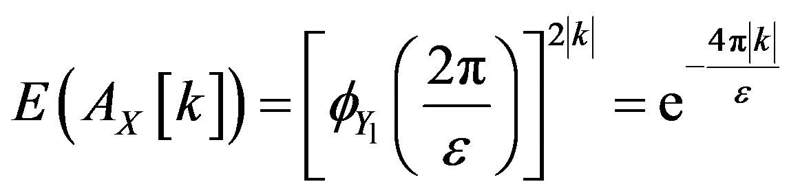
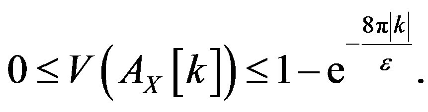
Theorem 2.5. Given  the waveform
  defined in (5) has autocorrelation
  such that
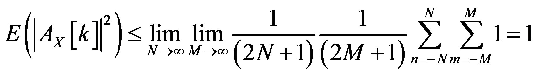
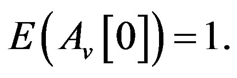
Proof. As defined in (6),
When 
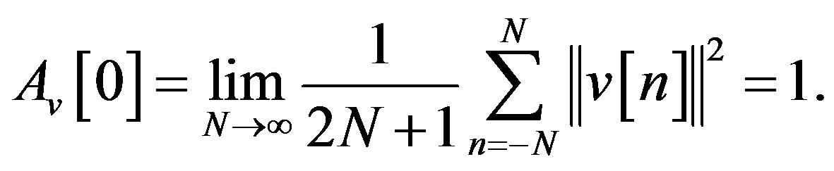
Thus,
For  due to (5),
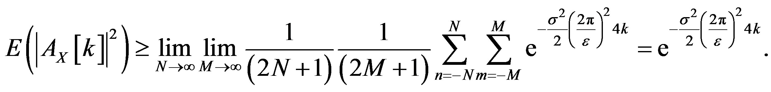
Consider 
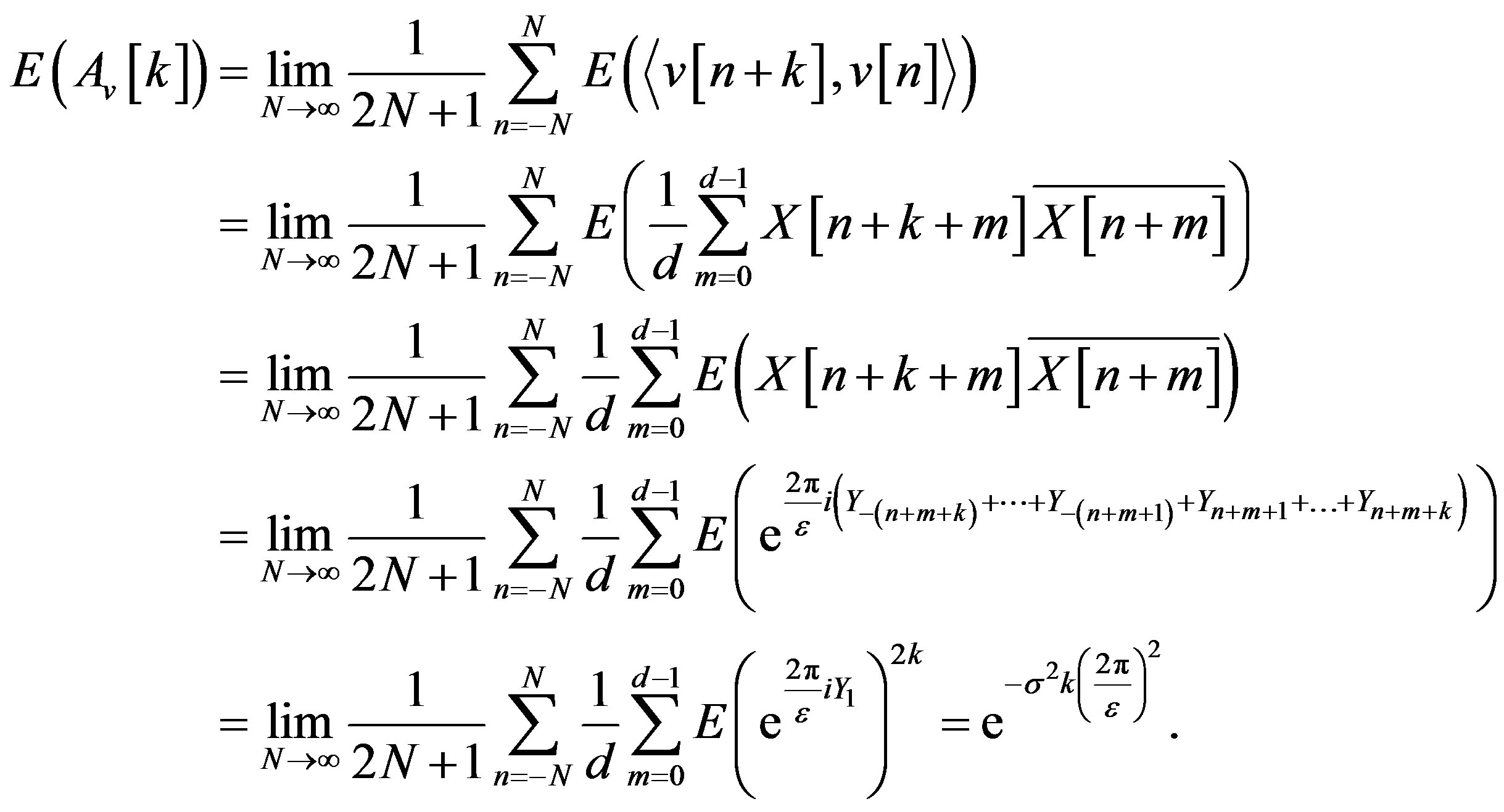
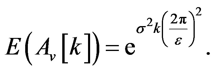
Similarly, for , one gets
 □
□
Thus the waveform  as defined in this section is unit-normed and has autocorrelation that can be made arbitrarily small.
Remark 2.6. As in the one dimensional construction, it is easy to see that here too the construction can be done with random variables other than the Gaussian. In fact, all random variables that can be used in the one dimensional case, i.e., ones satisfying the properties of Theorem 2.2, can also be used for the higher dimensional construction.
2.4. Remark on the Periodic Case
It can be shown that the periodic case follows the same nature as the aperiodic case. The sequence  is defined in the same way as in Section 2.1, i.e.,
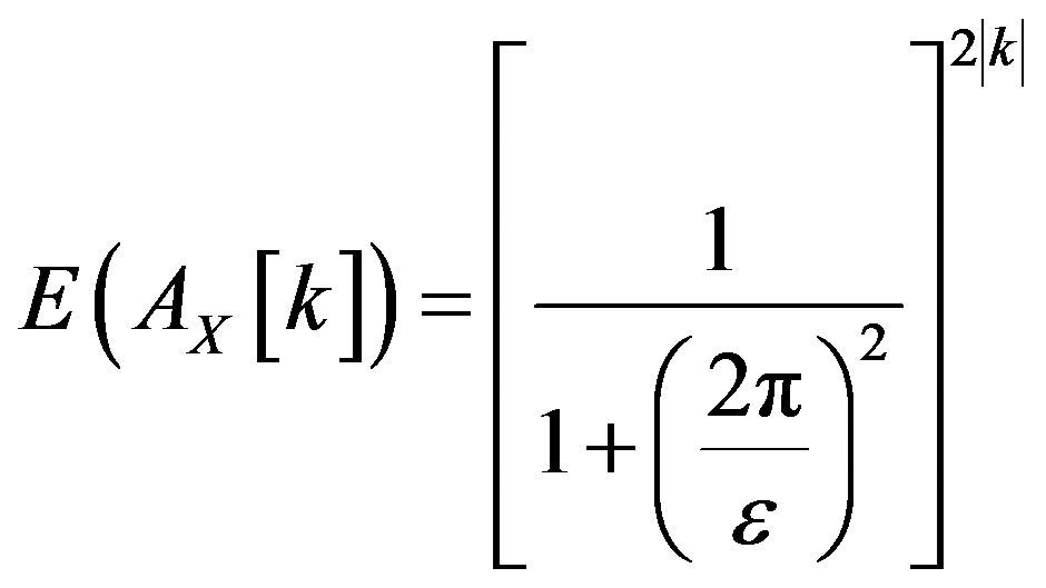
where 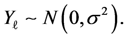 Following the definition given in (2), when
When  the expectation of the autocorrelation is
For 
where one uses the fact that the  s are i.i.d.. A similar calculation for negative values of k suggests that the autocorrelation can be made arbitrarily small, depending on
  for all non-zero values of k. Also, as in the aperiodic case, this result can be obtained for random variables other than the Gaussian.
3. Construction of Continuous Stochastic Waveforms
In this section continuous waveforms with almost perfect autocorrelation are constructed from a one dimensional Brownian motion.
For a continuous waveform , the autocorrelation
  can be defined as
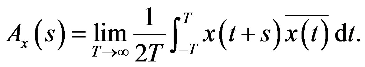 (7)
(7)
Let  be a one dimensional Brownian motion. Then
  satisfies
• 
• 
• 
 are independent random variables.
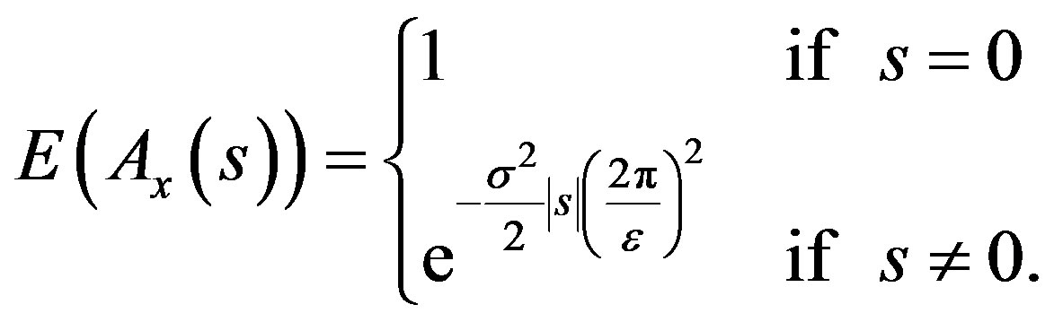
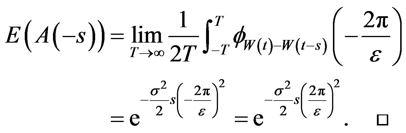
Theorem 3.1. Let  be the one dimensional Brownian motion and
  be given. Define
  by
by
and  Then the autocorrelation of
 satisfies
Proof. We would like to evaluate
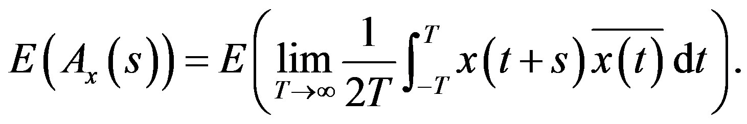
Let  and let
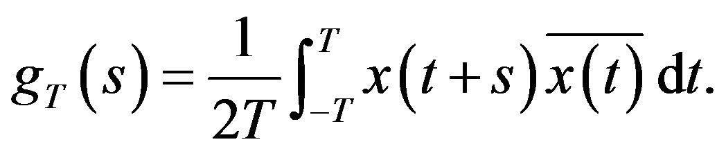
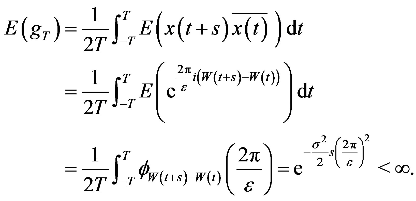
Thus each  is integrable and further
  Let
Let ;
; . Then
  Therefore, by the Dominated Convergence Theorem, and properties of Brownian motion and characteristic functions, one gets
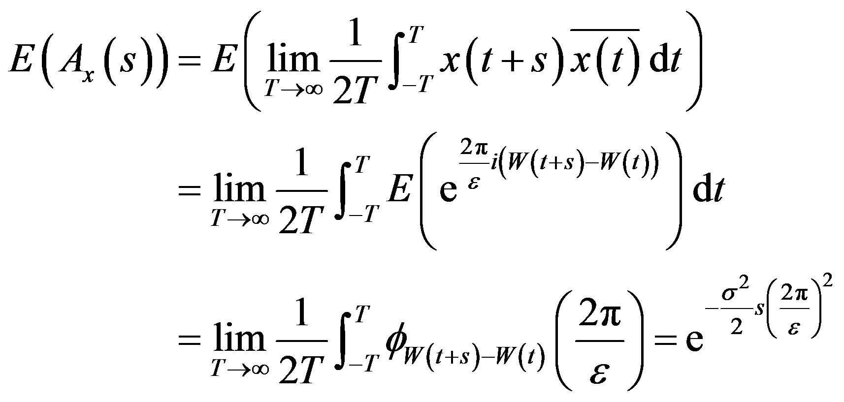
which can be made arbitrarily small based on  Similarly,
4. Connection to Frames
Consider the mapping  given by
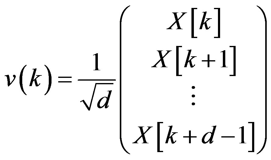 (8)
(8)
where 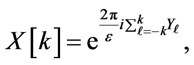 as defined in Section 2.1.
Let  and consider the set
  of
of  unit vectors in
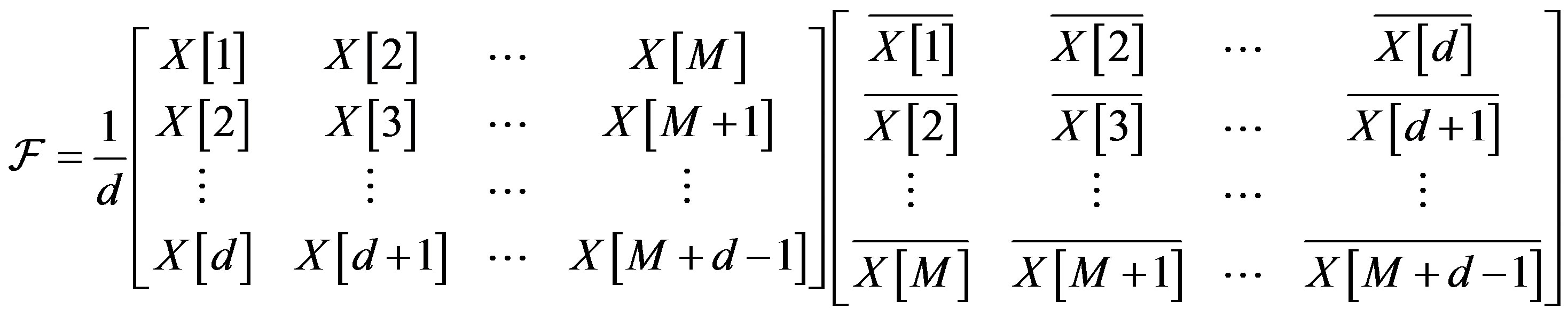
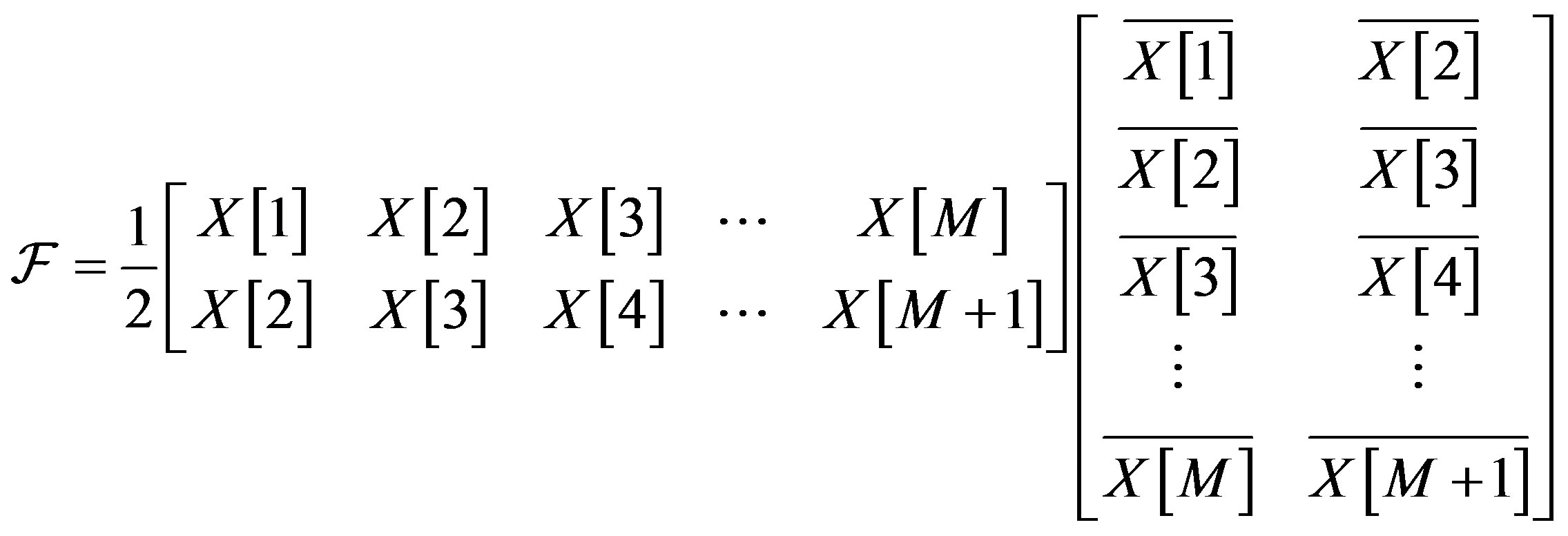
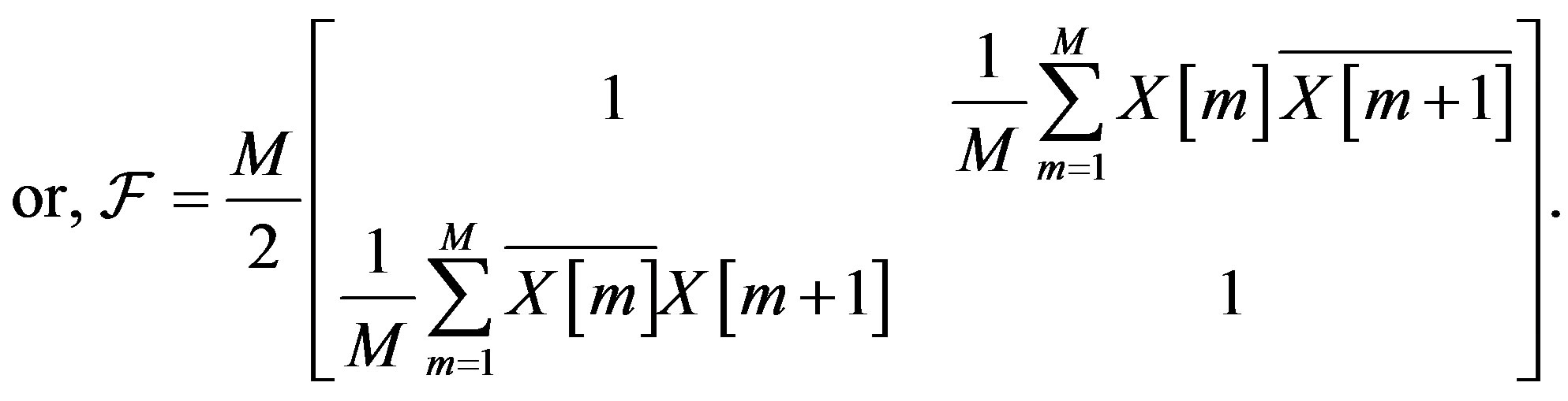
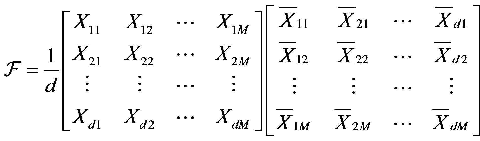
 . The matrix
is the matrix of the analysis operator corresponding to  The frame operator of
  is
is 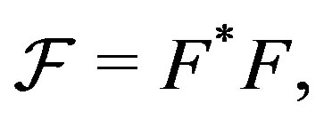 i.e.,
i.e.,
 .
.
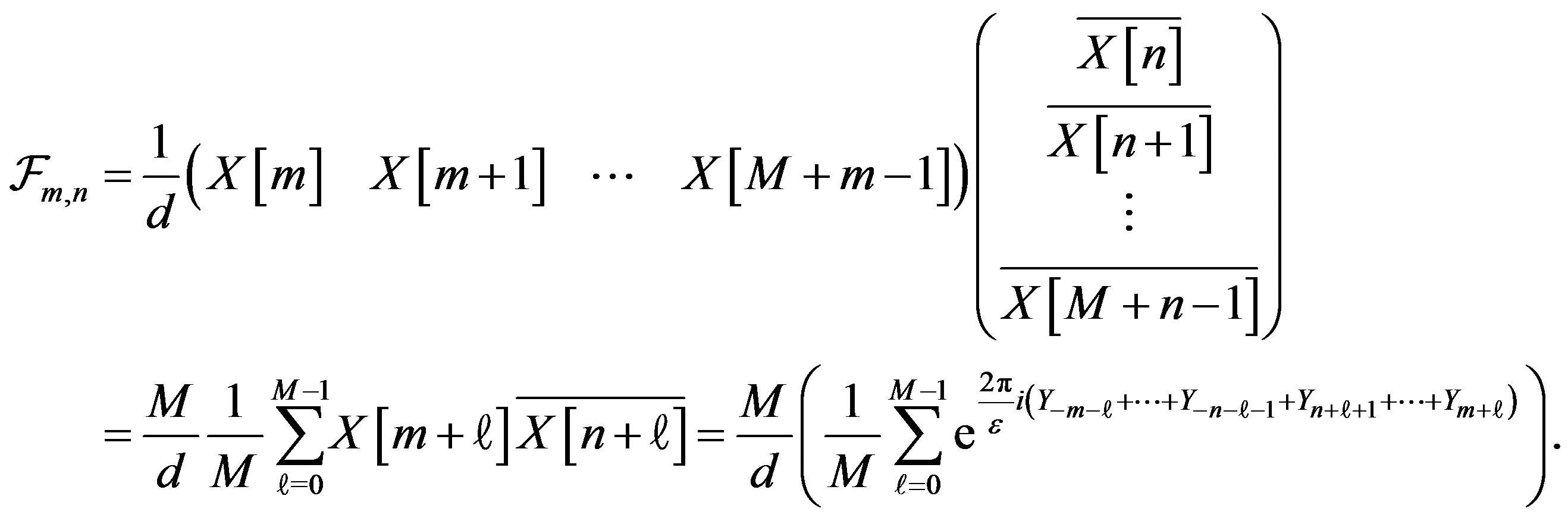
The entries of  are given by
 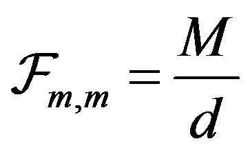 and for
Note that since  is self-adjoint,
 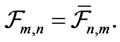 It is desired that V emulates a tight frame, i.e,
  is close to a constant times the identity, in this case,
  times the identity. Alternatively, it is desirable that the eigenvalues of
  are all close to each other and close to
 . In this case, due to the stochastic nature of the frame operator, one studies the expectation of the eigenvalues of
 .
.
4.1. Frames in 
This section discusses the construction of sets of vectors in  as given by (8). The frame properties of such sets are analyzed. In fact, it is shown that the expectation of the eigenvalues of the frame operator are close to each other, the closeness increasing with the size of the set. The bounds on the probability of deviation of the eigenvalues from the expected value is also derived. The related inequalities arise from an application of Theorem 4.1 [22] below.
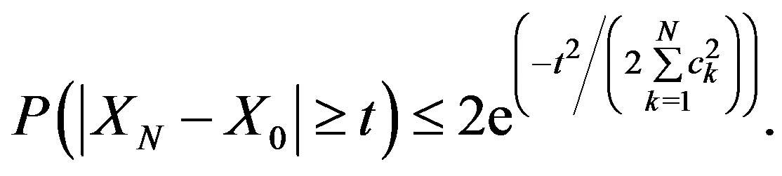
Theorem 4.1. (Azuma’s Inequality) Suppose that  is a martingale and
almost surely. Then for all positive integers  and all positive reals
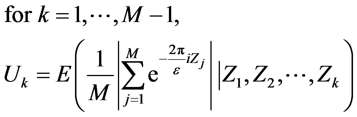
Consider  vectors in
  i.e.,
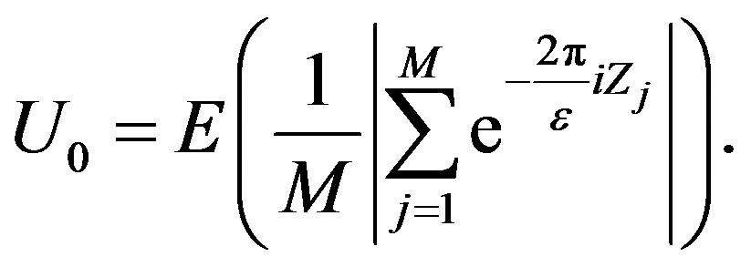
i.e.,  in (8). Then
  and
and
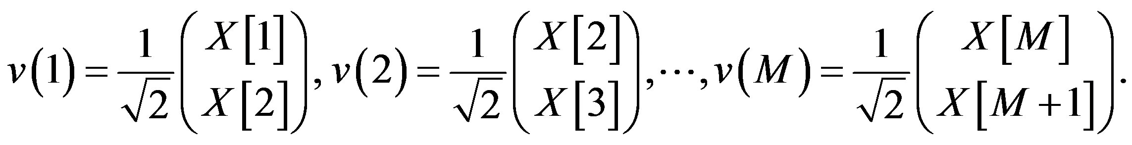 (9)
(9)
Considering the set  the frame operator of V is
 (10)
(10)
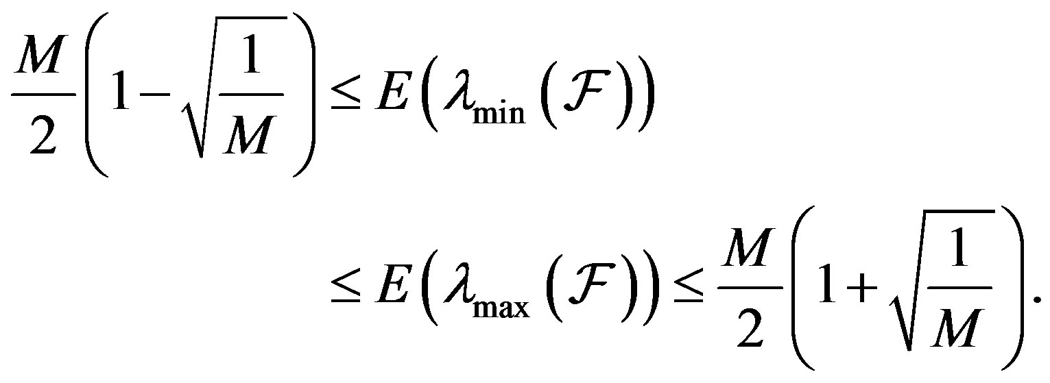
Theorem 4.2. 1) Consider the set 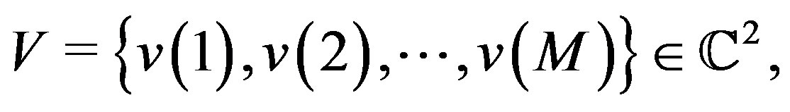
 where the vectors
  are given by (9). The minimum eigenvalue,
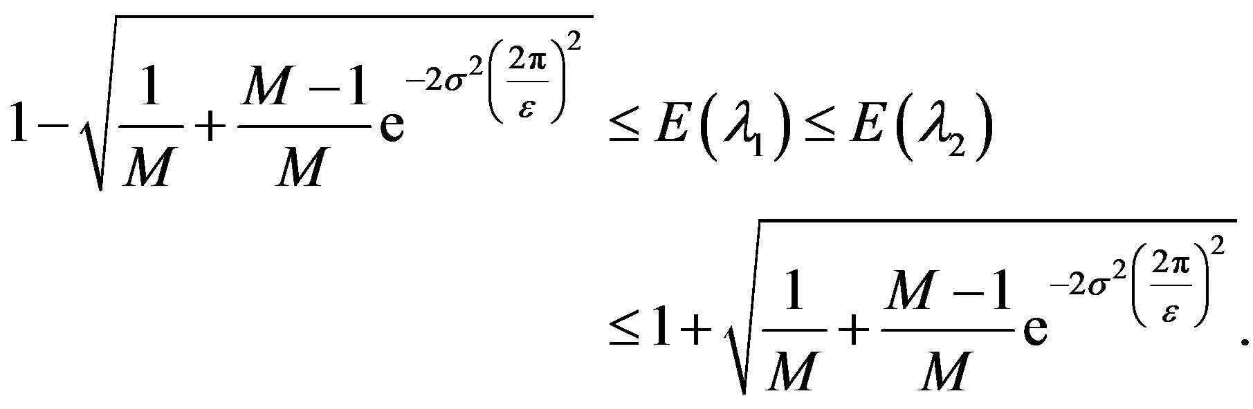
  and the maximum eigenvalue,
  of the frame operator of V satisfy
 (11)
(11)
where 
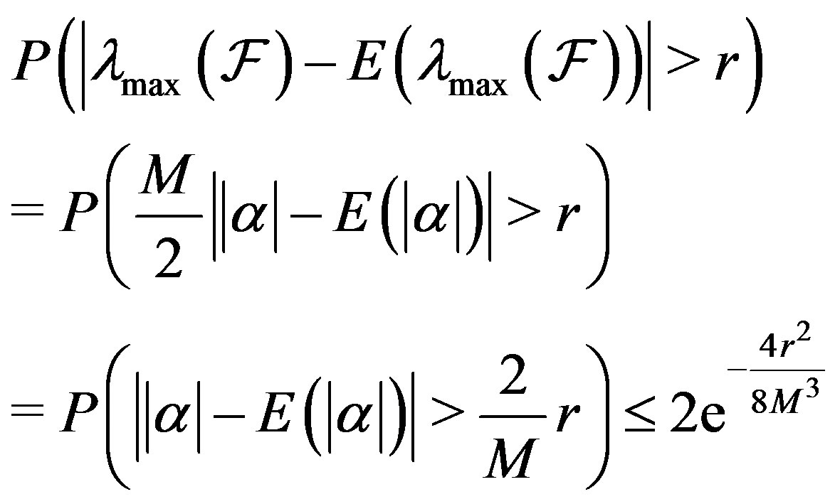
2) The deviation of the minimum and maximum eigenvalue of  from their expected value is given, for all positive reals
  by
by

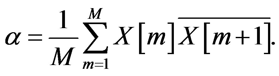
Proof. 1) The frame operator of
 is given in (10). The eigenvalues of
  are
are 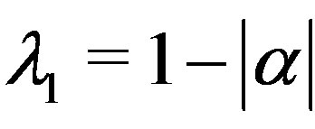 and
and 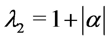 where
where
Let
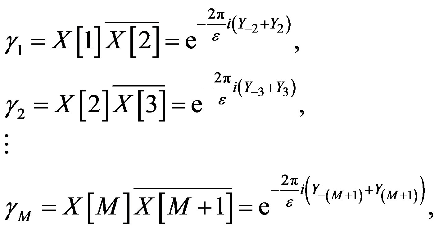
so that
Note that for 
 and
and  are independent and so
 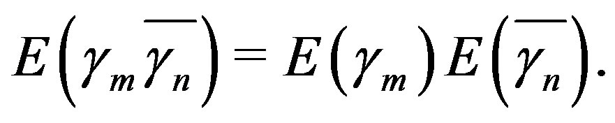 Also, since the
  s are i.i.d. and the characteristic function of the
  s is symmetric,
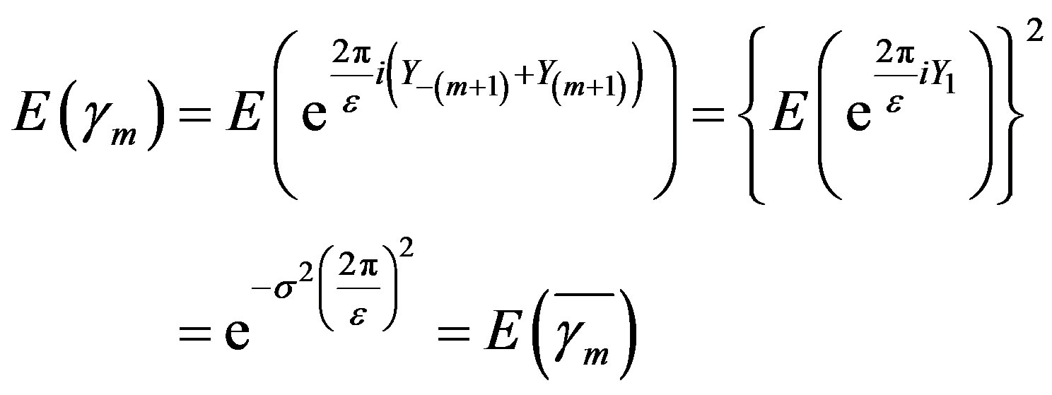
and therefore
Thus
The above estimate on  implies that
 (12)
(12)
Since  and
and , (12) implies
Noting that 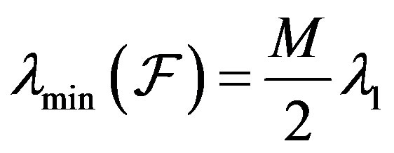 and
and  one finally gets, after setting
2) To prove 2) we use the Doob martingale and Azuma’s inequality [22]. For  let
let  Here the Doob martingale is the sequence
  where
where
and
Note that  and
and  Also,
Also,
So by Azuma’s Inequality (see Theorem 4.1)
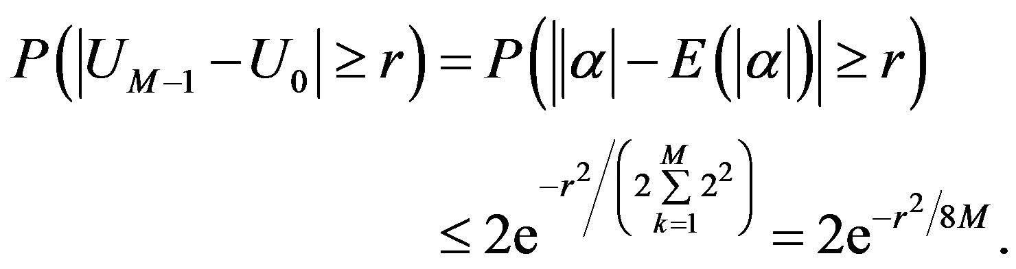
Since  this means
and
 .
.
Going back to the actual frame operator , whose eigenvalues are
  and
and  the following estimates hold.
and
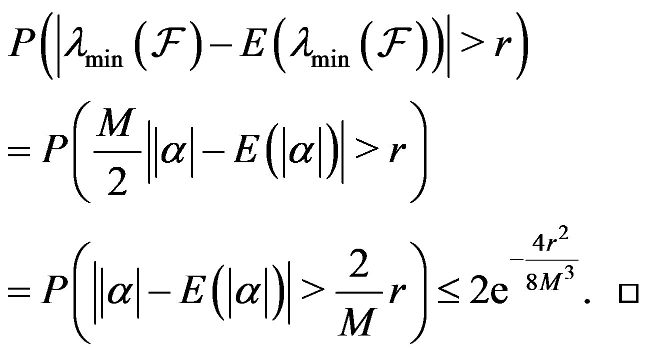
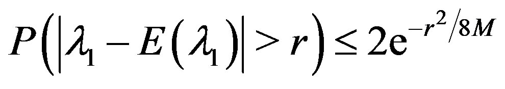
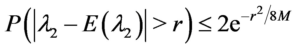
Corollary 4.3. The eigenvalues of the frame operator considered in Theorem 4.2 satisfy, for all positive reals r,
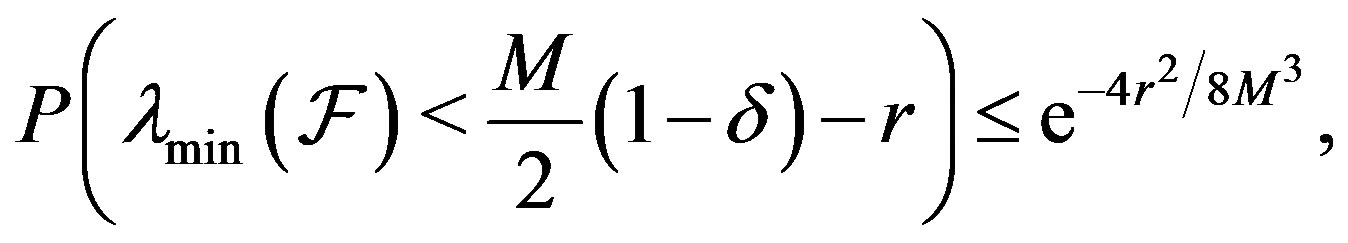
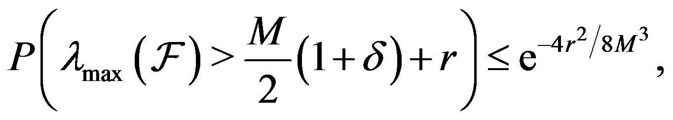
where 
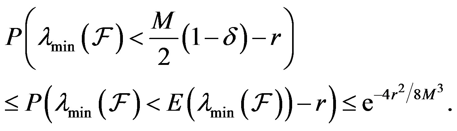
Proof. Due to part 1) of Theorem 4.2
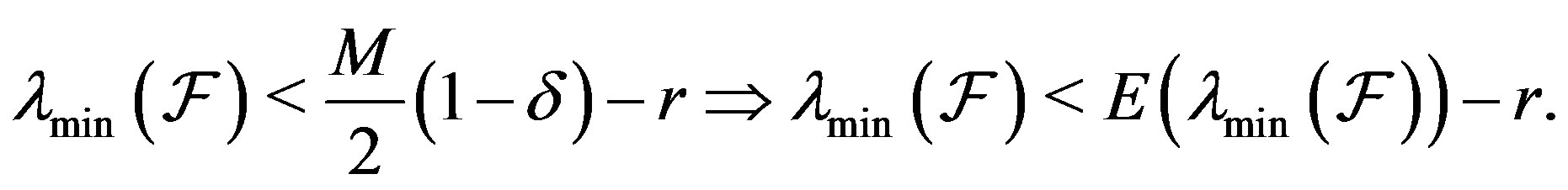
This implies, as a consequence of part 2) of Theorem 4.2, that
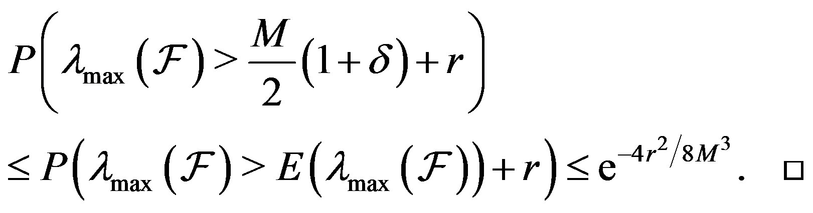
In a similar way, from part 1) of Theorem 4.2,
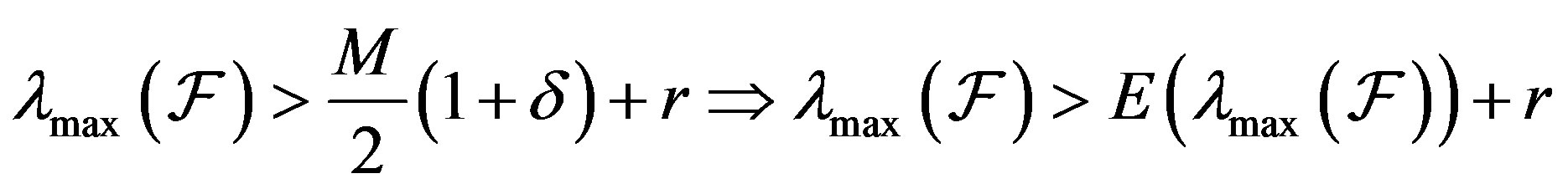
which implies, as a consequence of part 2) of Theorem 4.2, that
Remark 4.4. In Theorem 4.2, as M tends to infinity, the value of  in (11) can be made arbitrarily small based on the choice of
  This in turn implies that the two eigenvalues can be made arbitrarily close to each other, with
  On the other hand, for a fixed M, as
  tends to zero, (11) becomes
4.2. Frames in 
For general d and M, in order to use existing results on the concentration of eigenvalues of random matrices [23, 24], a slightly different construction of the frame needs to be considered. Let  be i.i.d. random variables following a Gaussian distribution with mean zero and variance
  It can be shown that
and the variance
One can define the following two dimensional sequence. For 
Consider the mapping  given by
 (13)
(13)
As before, let  and consider the set of
  unit vectors
  in
in . The frame operator of this set is
 .
.
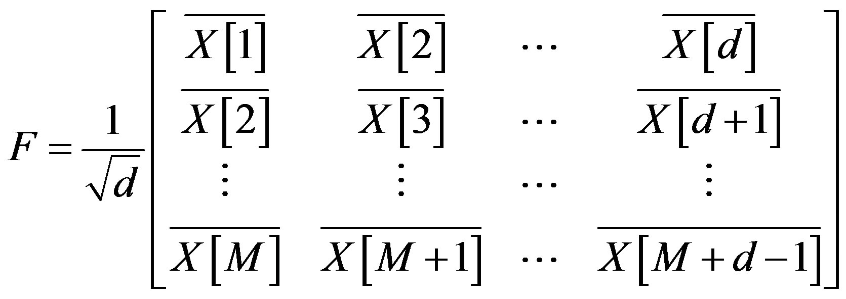
Let
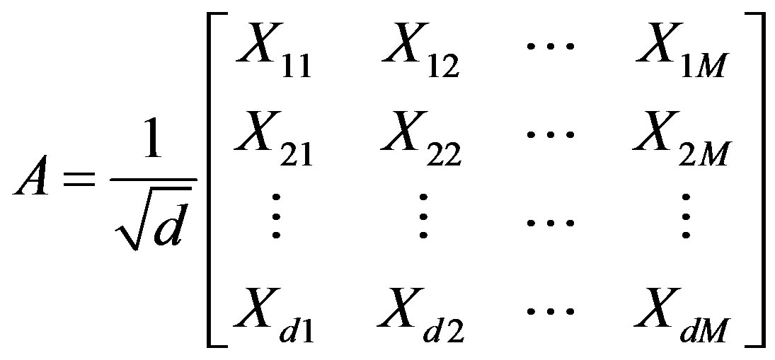 (14)
(14)
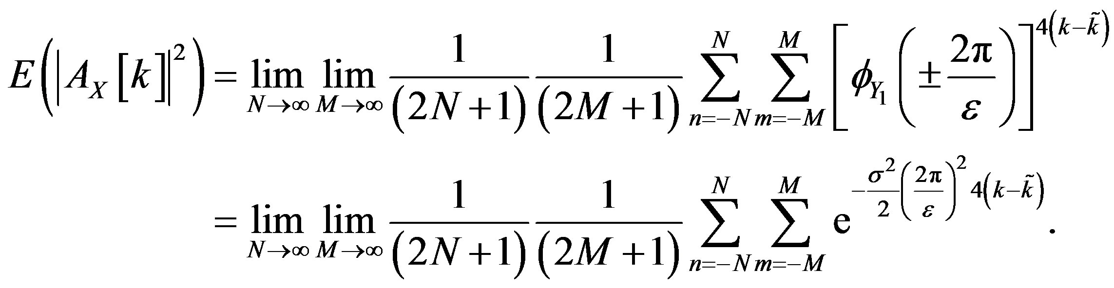
so that 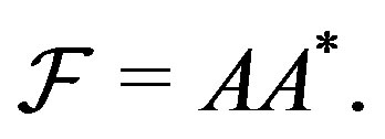 The matrix A has entries with mean zero and variance
 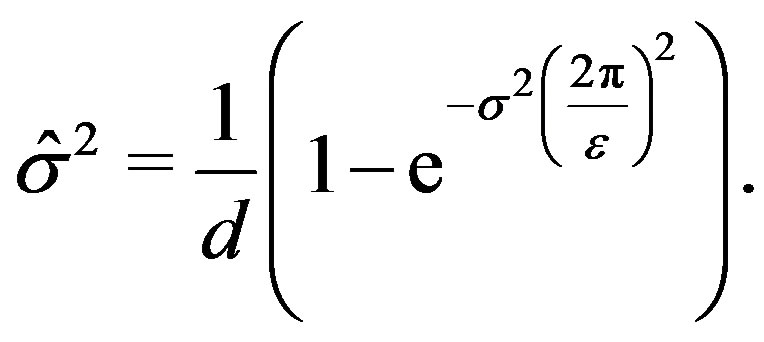 According to results in [23], if
 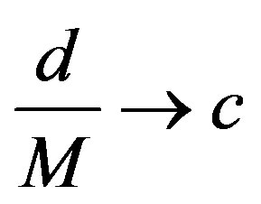 as
as 
 , then the smallest and largest eigenvalues of
  converge almost surely to
  and
and , respectively.
Theorem 4.5. Let  be the singular values of the matrix A given by (14). Then the following hold.
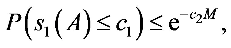
1) Given  there is a large enough d such that
 (15)
(15)
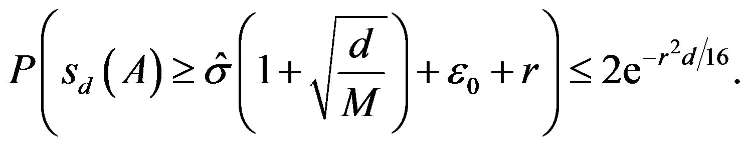
2)
 (16)
(16)
where  and
and  are universal positive constants.
Proof. Let  be the mapping that associates to a matrix
  it largest singular value. Equip
  with the Frobenius norm
Then the mapping  is convex and 1-Lipschitz in the sense that

for all pairs  of d by M matrices [24].
We think of A as a random vector in  The real and imaginary parts of the entries of
  are supported in
  Let P be a product measure on
 . Then as a consequence of the concentration inequality (Corollary 4.10, [24]) we have
where  is the median of
 . It is known that the minimum and maximum singular values of A converge almost surely to
  and
and , respectively, as d, M tend to infinity and
 . As a consequence, for each
  and M sufficiently large, one can show that the medians belong to the fixed interval
 which gives

For the smallest singular value we cannot use the concentration inequality as used for  since the smallest singular value is not convex. However, following results in [25] (Theorem 3.1) that have been used in [26] in a similar situation as here, one can say that whenever
 , where
  is greater than a small constant,
 where
where  and
and  are positive universal constants. □
Remark 4.6. Note that the square of the singular values of A are the eigenvalues of  and so the estimates given in (15) and (16) give insight into the corresponding deviation of the eigenvalues of the frame operator
 .
.
Remark 4.7. (Connection to compressed sensing) The theory of compressed sensing [27-29] states that it is possible to recover a sparse signal from a small number of measurements. A signal  is k-sparse in a basis
 if x is a weighted superposition of at most k elements of
 . Compressed sensing broadly refers to the inverse problem of reconstructing such a signal x from linear measurements
  with
with , ideally with
 . In the general setting, one has
 , where
  is a
is a  sensing matrix having the measurement vectors
  as its columns, x is a length-M signal and y is a length-d measurement.
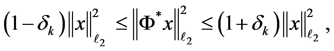
The standard compressed sensing technique guarantees exact recovery of the original signal with very high probability if the sensing matrix satisfies the Restricted Isometry Property (RIP). This means that for a fixed k, there exists a small number , such that
for any k-sparse signal x. By imitating the work done in [26] (Lemmas 4.1 and 4.2), it can be shown, due to Theorem 4.5, that matrices A of the type given in (14) satisfy
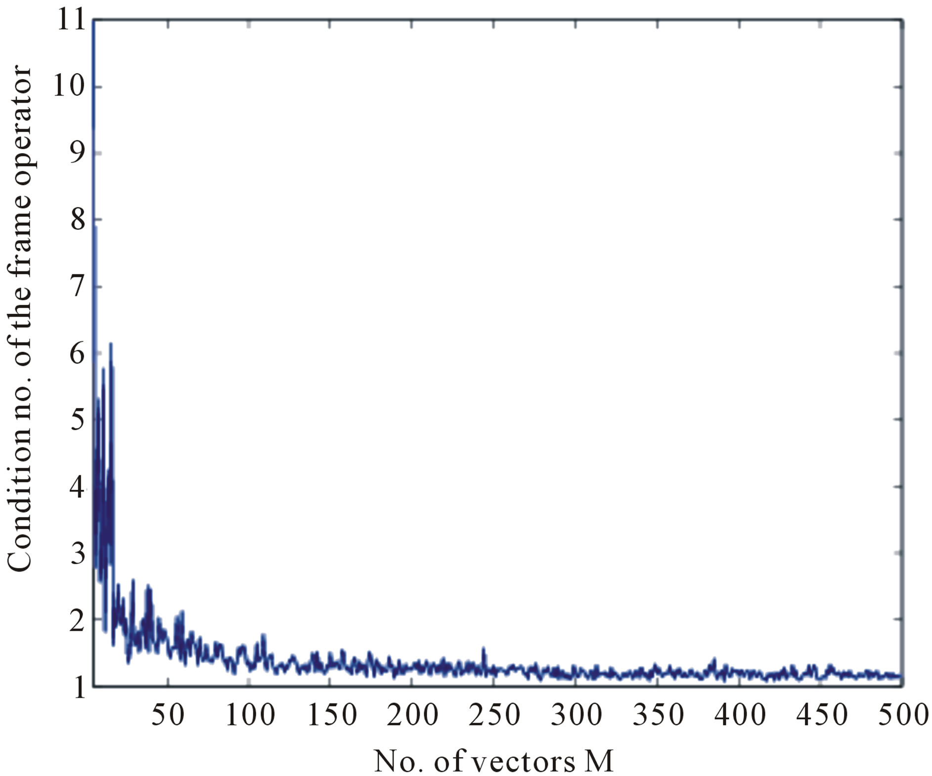
Figure 1. Behavior of the condition number of the frame operator with increasing size of the frame; ε = 0.0001, d = 3, σ = 1.
the RIP condition and can therefore be used as measurement matrices in compressed sensing. These matrices are different from the traditional random matrices used in compressed sensing in that their entries are complexvalued and unimodular instead of being real-valued and not unimodular.
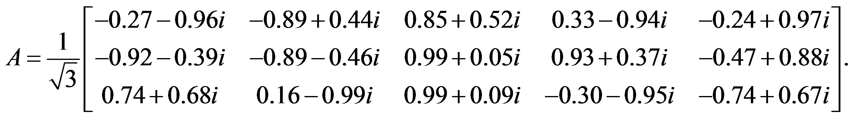
Example 4.8. This example illustrates the ideas in this subsection. First consider M = 5 and d = 3 so that there are 5 vectors in  Taking from a normal distribution with mean 0 and variance
  a realization of the matrix
  is
is
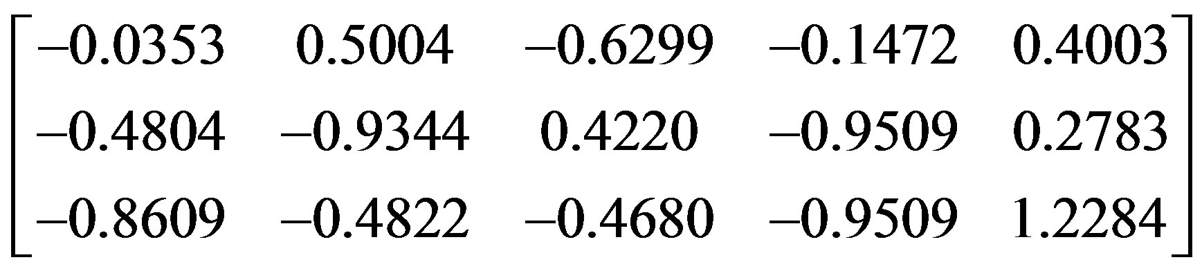 .
.
Then taking 
 is
is
The condition number, ratio of the maximum and minimum eigenvalues, of  As the number of vectors M is increased, the condition number gets closer to 1. Figure 1 shows the behavior of the condition number with the increase in the number of vectors.
5. Conclusion
The construction of discrete unimodular stochastic waveforms with arbitrarily small expected autocorrelation has been proposed. This is motivated by the usefulness of such waveforms in the areas of radar and communications. The family of random variables that can be used for this purpose has been characterized. Such construction been done in one dimension and generalized to higher dimensions. Further, such waveforms have been used to construct frames in  and the frame properties of such frames have been studied. Using Brownian motion, this idea is also extended to the construction of continuous unimodular stochastic waveforms whose autocorrelation can be made arbitrarily small in expectation.
6. Acknowledgements
The author wishes to acknowledge support from AFOSR Grant No. FA9550-10-1-0441 for conducting this research. The author is also grateful to Frank Gao and Ross Richardson for their generous help with probability theory.
REFERENCES
- L. Auslander and P. E. Barbano, “Communication Codes and Bernoulli Transformations,” Applied and Computational Harmonic Analysis, Vol. 5, No. 2, 1998, pp. 109- 128. doi:10.1006/acha.1997.0222
- J. J. Benedetto and J. J. Donatelli, “Ambiguity Function and Frame Theoretic Properties of Periodic Zero Autocorrelation Waveforms,” IEEE Journal of Selected Topics in Signal Processing, Vol. 1, 2007, pp. 6-20.
- T. Helleseth and P. V. Kumar, “Sequences with Low Correlation,” Handbook of Coding Theory, North-Holland, Amsterdam, 1998, pp. 1765-1853.
- N. Levanon and E. Mozeson, “Radar Signals,” Wiley Interscience, New York, 2004. doi:10.1002/0471663085
- M. L. Long, “Radar Reflectivity of Land and Sea,” Artech House, 2001.
- W. H. Mow, “A New Unified Construction of Perfect Root-of-Unity Sequences,” Proceedings of IEEE 4th International Symposium on Spread Spectrum Techniques and Applications, Sun City, 22-25 September 1996, pp. 955-959. doi:10.1109/ISSSTA.1996.563445
- F. E. Nathanson, “Radar Design Principles: Signal Processing and the Environment,” SciTech Publishing Inc., Mendham, 1999.
- G. W. Stimson, “Introduction to Airborne Radar,” SciTech Publishing Inc., Mendham, 1998.
- S. Ulukus and R. D. Yates, “Iterative Construction of Optimum Signature Sequence Sets in Synchronous CDMA Systems,” IEEE Transactions on Information Theory, Vol. 47, No. 5, 2001, pp. 1989-1998. doi:10.1109/18.930932
- S. Verdú, “Multiuser Detection,” Cambridge University Press, Cambridge, 1998.
- J. J. Benedetto and S. Datta, “Construction of Infinite Unimodular Sequences with Zero Autocorrelation,” Advances in Computational Mathematics, Vol. 32, No. 2, 2010, pp. 191-207. doi:10.1007/s10444-008-9100-9
- D. Cochran, “Waveform-Agile Sensing: Opportunities and Challenges,” IEEE International Conference on Acoustics, Speech, and Signal Processing, Pennsylvania, 18-23 March 2005, pp. 877-880.
- M. R. Bell, “Information Theory and Radar Waveform Design,” IEEE Transactions on Information Theory, Vol. 39, No. 5, 1993, pp. 1578-1597. doi:10.1109/18.259642
- S. P. Sira, Y. Li, A. Papandreou-Suppappola, D. Morrell, D. Cochran and M. Rangaswamy, “Waveform-Agile Sensing for Tracking,” IEEE of Signal Processing Magazine, Vol. 26, No. 1, 2009, pp. 53-64.
- H. Boche and S. Stanczak, “Estimation of Deviations between the Aperiodic and Periodic Correlation Functions of Polyphase Sequences in Vicinity of the Zero Shift,” IEEE 6th International Symposium on Spread Spectrum Techniques and Applications, Parsippany, 6-8 September 2000, pp. 283-287.
- R. Narayanan, “Through Wall Radar Imaging Using UWB Noise Waveforms,” IEEE International Conference on Acoustics, Speech and Signal Processing, Beijing, 31 March-4 April 2008, pp. 5185-5188.
- R. M. Narayanan, Y. Xu, P. D. Hoffmeyer and J. O. Curtis, “Design, Performance, and Applications of a Coherent Ultra-Wideband Random Noise Radar,” Optical Engineering, Vol. 37, No. 6, 1998, pp. 1855-1869.
- D. Bell and R. Narayanan, “Theoretical Aspects of Radar Imaging Using Stochastic Waveforms,” IEEE Transactions on Signal Processing, Vol. 49, No. 2, 2001, pp. 394-400. doi:10.1109/78.902122
- A. F. Karr, “Probability of Springer Texts in Statistics,” Springer-Verlag, New York, 1993.
- O. Christensen, “An Introduction to Frames and Riesz Bases,” Birkhäuser, 2003.
- I. Daubechies, “Ten Lectures on Wavelets,” CBMS-NSF Regional Conference Series in Applied Mathematics, 1992. doi:10.1137/1.9781611970104
- W. Hoeffding, “Probability Inequalities for Sums of Bounded Random Variables,” Journal of American Statistical Association, Vol. 58, No. 301, 1963, pp. 13-30. doi:10.1080/01621459.1963.10500830
- Z. D. Bai, “Methodologies in Spectral Analysis of LargeDimensional Random Matrices: A Review,” Statistica Sinica, Vol. 9, No. 3, 1999, pp. 611-677.
- M. Ledoux, “The Concentration of Measure Phenomenon,” Mathematical Surveys and Monographs, American Mathematical Society, 2001.
- A. E. Litvak, A. Pajor, M. Rudelson and N. TomczakJaegermann, “Smallest Singular Value of Random Matrices and Geometry of Random Polytopes,” Advances in Mathematics, Vol. 195, No. 2, 2005, pp. 491-523. doi:10.1016/j.aim.2004.08.004
- E. Candès and T. Tao, “Near Optimal Signal Recovery from Random Projections: Universal Encoding Strategies?” IEEE Transactions on Information Theory, Vol. 52, No. 12, 2006, pp. 5406-5425. doi:10.1109/TIT.2006.885507
- E. Candès, “Compressive Sampling,” Proceedings of the International Congress of Mathematicians, Madrid, 22-30 August 2006, pp. 1433-1452.
- E. Candès, J. Romberg and T. Tao, “Robust Uncertainty Principles: Exact Signal Reconstruction from Highly Incomplete Frequency Information,” IEEE Transactions on Information Theory, Vol. 52, No. 2, 2006, pp. 489-509. doi:10.1109/TIT.2005.862083
- D. L. Donoho, “Compressed Sensing,” IEEE Transactions on Information Theory, Vol. 52, No. 4, 2006, pp. 1289- 1306. doi:10.1109/TIT.2006.871582
NOTES
*This work was supported by AFOSR Grant No. FA9550-10-1-0441.