Agricultural Sciences
Vol.3 No.4(2012), Article ID:20096,12 pages DOI:10.4236/as.2012.34065
Diffusion models for the description of seedless grape drying using analytical and numerical solutions
![]()
Federal University of Campina Grande, Campina Grande, Brazil; *Corresponding Author: wiltonps@uol.com.br
Received 20 March 2012; revised 26 April 2012; accepted 2 May 2012
Keywords: Optimization; Convective Boundary Condition; Diffusion Model; Finite Volume Method
ABSTRACT
This article compares diffusion models used to describe seedless grape drying at low temperature. The models were analyzed, assuming the following characteristics of the drying process: boundary conditions of the first and the third kind; constant and variable volume, V; constant and variable effective mass diffusivity, D; constant convective mass transfer coefficient, h. Solutions of the diffusion equation (analytical and numerical) were used to determine D and h for experimental data of seedless grape drying. Comparison of simulations of drying kinetics indicates that the best model should consider: 1) shrinkage; 2) convective boundary condition; 3) variable effective mass diffusivity. For the analyzed experimental dataset, the best function to represent the effective mass diffusivity is a hyperbolic cosine. In this case, the statistical indicators of the simulation can be considered excellent (the determination coefficient is R2 = 0.9999 and the chi-square is χ2 = 3.241 × 10⁻⁴).
1. INTRODUCTION
After harvest, the time of fruit conservation under natural conditions is limited to only a few days. Grapes, for instance, belong to the most perishable fruits. They are very susceptible to microbial decay and moisture loss. In general, two mechanisms are used to prolong the consuming time of grapes: cooling and drying. In the second case, the life time of the product is much higher than in the first case, beyond resulting in a food very appreciated in several parts of the world: raisins. The drying process of grapes under natural conditions [1] is generally slow due to the resistance of its skin. In order to increase the drying rate, commonly a pretreatment is accomplished before drying. Several pretreatment techniques involving the use of chemical additives are described in the literature [2-6]. However, the demand for natural foods, without adding chemicals, is increasing in many parts of the world. Therefore, alternatives to chemical additives are used as pretreatment for the production of raisins, for instance: abrasion method [7] and dipping in hot water [6, 8].
For describing the drying process, a mathematical model must be used. Several drying models are available in the literature: empirical models [1-5], and diffusion models, which are very common to describe drying kinetics of grapes [1,3,4-9]. In order to describe the drying kinetics through a diffusion model, the initial and boundary conditions must be known. In general, the appropriate boundary condition is of the third kind [6,7,9], but the first kind one is also found in several research works [1, 3-6,8], especially if some pretreatment is used before the drying process. For some products, like rice, drying does not substantially reduce the volume of the product and the shrinkage can be discarded [10,11]. However, in products such as banana [12] and grape [6,8], the shrinkage is so significant that its effect should not be discarded. But if shrinkage is taken into account, its effect on the diffusivity should also be considered: the effective mass diffusivity should have a variable value throughout the process [6,8].
If a diffusion model is used to describe the drying of a product, the diffusion equation must be solved. Some research works present analytical solutions for the diffusion equation, particularly if the boundary condition is of the first kind [1,3-7]. If an analytical solution is proposed for the boundary condition of the third kind, the series which represents the solution is normally expressed by only the first term, and the process parameters are determined by regression [13,14]. However, this procedure only works well with experimental data referring to Fourier numbers grater than 0.2. For the boundary condition of the third kind, numerical solutions are frequently found in the literature, if the complete drying kinetic must be studied [9,15-20].
In order to use the aforementioned solutions for the description of seedless grape drying, the process parameters must be known. These parameters can be determined through optimization processes, normally by using the inverse method [21,22]. Once the process parameters are known, the simulation of the drying kinetics can be performed, and the moisture content can be determined at an instant t in any position r within the grape.
Since several models are available in the literature to describe the drying of grapes, this article investigates what is the most appropriate one. To this end, five diffusion models, involving the aspects discussed above, were used to describe seedless grape drying. Then, the results for each model were compared with each other and the best model was determined.
2. MATERIAL AND METHODS
The solutions of the diffusion equation to describe seedless grape drying presupposes the following hypotheses: 1) grapes are considered as spheres; 2) grapes are considered as homogeneous and isotropic; 3) the moisture distribution inside the grapes must present radial symmetry and must be initially uniform; 4) the convective mass transfer coefficient is constant; 5) diffusion is the only mass transport mechanism inside the grapes.
2.1. Diffusion Equation and Boundary Condition
Given the hypotheses above, the one-dimensional moisture diffusion equation can be written in spherical coordinates as
 (1)
(1)
where M is the moisture content (db), r defines the position inside the sphere (m), D is the effective mass diffusivity (m·s–1), and t is the time (s).
The boundary condition of the third kind may be expressed by the equation:
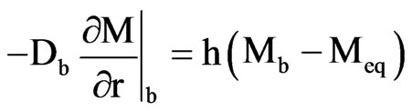 (2)
(2)
where h is the convective mass transfer coefficient (m·s–1),  is the moisture content at the boundary (db), and
  is the equilibrium moisture content (db).
2.2. Analytical Solution
The analytical solution presented in this article refers to a spherical geometry governed by Eqs.1 and 2, where a constant value for the effective mass diffusivity D is assumed. For a sphere with radius R and an initial moisture content M0, the solution M(r,t) of Eq.1 with boundary condition given by Eq.2 is [23,24]:
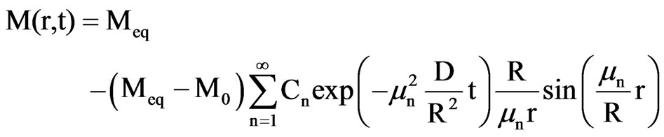 (3)
(3)
with
 (4)
(4)
where  are roots of a characteristic equation to be defined later. In Eq.3, M(r,t) is the moisture content (dry basis) at the position r from the centre of the sphere at time t.
The average value of the moisture content at time t is defined by
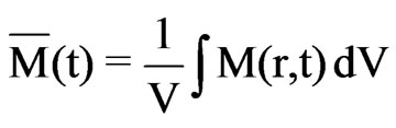 (5)
(5)
The solution of the diffusion equation for the average value  of a spherical body is obtained by substituting Eq.3 into Eq.5, and the result is:
 (6)
(6)
where
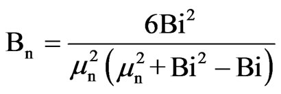 (7)
(7)
Here, Bi is the Biot number given by
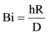 (8)
(8)
and  are the roots of the characteristic equation for the sphere
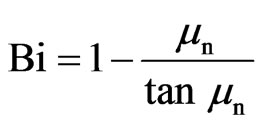 (9)
(9)
If only the experimental data corresponding to a Fourier number Fo = Dt/R2 > 0.2 are analyzed, the drying kinetic is well described by the first term of the sum in Eq.6 [14]. Using the dimensionless moisture content,
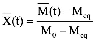 (10)
(10)
Eq.6 reduces for this situation to
 (11)
(11)
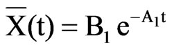
where  is given by Eq.7, with n = 1, and
 (12)
(12)
Then, the parameters B1 and A1 can be determined by fit Eq.11 to experimental data. By substitution of Eq.9 into Eq.7, with n = 1, a transcendental equation is obtained, and the root , corresponding to n = 1, can be determined. Thus, the Biot number is also determined through Eq.9, and the effective mass diffusivity by Eq.12. Once Bi and D are known, Eq.8 can be used to calculate the convective mass transfer coefficient, h.
2.3. Numerical Solution
Eq.1 was also numerically solved by using the finite volume method with fully implicit formulation [20,25]. Figure 1 presents the uniform one-dimensional mesh of the corresponding sphere. The control volumes have a thickness  (m) and the control volume number “i” has a nodal point “P”.
Integration of Eq.1 over space ( ) and time (
 ) gives the following result for the control volume P:
 (13)
(13)
where the superscript “0” means “former time t” and its absence means “current time t + Dt”. The indexes “P”, “e” and “w” refer, respectively, to the nodal point, and east and west interfaces of the control volume.
Discretizing Eq.2 gives
 (14)
(14)
and therefore
 (15)
(15)
where the subscript b refers to the boundary.
For an internal control volume (control volume from 2 up to N – 1), Eq.13 results in:
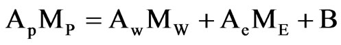 (16)
(16)
where
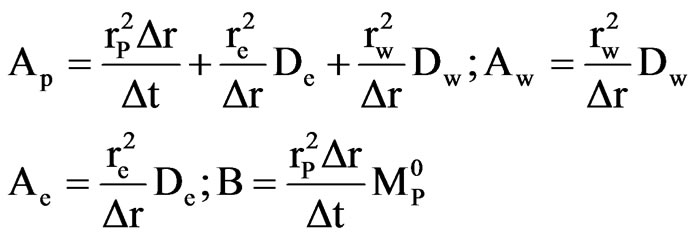 (17)
(17)
For the control volume 1, due to the symmetry condition (flux zero at the centre), Eq.13 becomes:
 (18)
(18)

Figure 1. (a) Uniform mesh: N control volumes with thickness Δr; (b) Control volume P and its neighbors to west (W) and to east (E).
with
 (19)
(19)
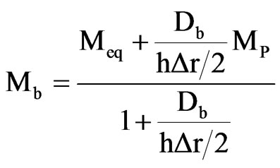
For the control volume N (boundary), the combination of Eqs.13 and 14 results in:
 (20)
(20)
with
 (21)
(21)
Considering the numerical solution, the system of Eqs.16, 18 and 20 can be solved for each time step, for instance, by the TDMA method (Press et al., 1996). Note that the coefficients A are calculated only once if the effective mass diffusivity D is constant, whereas B is calculated in each time step because its value depends on , the moisture content of the control volume P at the beginning of each time step. Otherwise, if the effective mass diffusivity is variable, the coefficients A also must be calculated in each time step, due to the nonlinearities caused by the variation of D. In this case, errors due to these nonlinearities can be eliminated by adequate time refinement. As the volume of the fruit is variable during the process, the position r of each nodal point must be recalculated in each time step. Once
  is numerically determined, the moisture content Mb (at the boundary) can be calculated from Eq.15 at a given time t.
The average value of M at a given time t may be calculated by Eq.5, written in the discretized form [20]:
 (22)
(22)
where Vj are the volumes of the control volume “j” (m3) and
 (23)
(23)
is the volume of the sphere (m3).
2.4. Effective Mass Diffusivity
In case of the numerical solution, the process parameter D may be calculated at nodal points from an appropriate relation between D and the moisture content M (or dimensionless moisture content X):
 (24)
(24)
where “a” and “b” are parameters which fit the numerical solution to the experimental data, and they are determined by optimization.
At the interfaces between control volumes, for example “e” (Figure 1), a harmonic mean given by the following expression must be used to determine  [20, 25]:
 (25)
(25)
which is valid for uniform grids. Note that Eq.25 is also valid for a constant effective mass diffusivity, with a value D. In this case,  ,
, ; and Eq.25 becomes
 .
.
2.5. Optimization
The expression for the chi-square involving the fit of a simulated curve to the experimental data was used as objective function, and is given by [26,27]
 (26)
(26)
where  is the moisture content measured at the experimental point “i” (db),
  is the correspondent simulated moisture content (db), Np is the number of experimental points,
  is the statistical weight referring to the point “i”. If the statistical weights are not known, they are set equal to 1. In Eq.26, the chi-square depends on
 , which depends on D and h. If h can be considered as constant and the effective mass diffusivity is given by Eq.24, the parameters a, b and h can be determined through the minimization of the objective function, which can be accomplished in cycles involving the following steps:
Step 1. Inform the initial values for the parameters “a”, “b” and “h”. Solve the diffusion equation and determine the chi-square;
Step 2. Inform the value for the correction of “h”;
Step 3. Correct the parameter “h”, keeping the parameters “a” and “b” constant. Solve the diffusion equation and calculate the chi-square;
Step 4. Compare the last calculated value of the chisquare with the previous one. If the last value is smaller, return to the step 2; otherwise, decrease the last correction of the value of “h” and proceed with step 5;
Step 5. Inform the value for the correction of “a”;
Step 6. Correct the parameter “a”, keeping the parameters “b” and “h” constant. Solve the diffusion equation and calculate the chi-square;
Step 7. Compare the last calculated value of the chisquare with the previous one. If the last value is smaller, return to step 5; otherwise, decrease the last correction of the value of “a” and proceed with step 8;
Step 8. Inform the value for the correction of “b”;
Step 9. Correct the parameter “b”, keeping the parameters “a” and “h” constant. Solve the diffusion equation and calculate the chi-square;
Step 10. Compare the last calculated value of the chisquare with the previous one. If the last value is smaller, return to the step 8; otherwise, decrease the last correction of the value of “b” and proceed with step 11;
Step 11. Begin a new cycle going back to step 2 until the stipulated convergence for the parameters “a”, “b” and “h” is reached.
In each cycle, the value of the correction of each parameter can be initially modest, compatible with the tolerance of convergence imposed to the problem. Then, for a given cycle, in each return to step 2, 5 or 8, the value of the new correction can be multiplied by the factor 2. If the initially informed modest correction does not minimize the objective function, its value can be multiplied by the factor –1 in the next cycle. Note that the steps 8, 9 and 10 are not necessary when the effective mass diffusivity is supposed to be constant. Initial values for the parameters can be estimated through values obtained from similar products available in the literature, or through empirical correlations.
2.6. Software
The software used to determine h and D through numerical solution was developed in an Intel Pentium IV computer with 1 GB RAM. The program was compiled in Compaq Visual Fortran (CVF) 6.6.0 Professional Edition, using the programming option QuickWin Application, in a Windows XP platform. The developed software was also used to draw contour plots at specified times, showing the moisture content distribution within the sphere which represents the grape. Besides these characteristics, the software also draws the numerically simulated curve, which was fitted to the experimental data. The statistical indicators used in the analyses of the obtained results were chi-square , and determination coefficient R2 [26,27]. LAB Fit Curve Fitting Software V. 7.2.48 (http://zeus.df.ufcg.edu.br/labfit) was used for the statistical treatment of the data.
2.7. Experimental Data
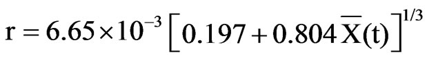
Experimental data obtained by Esmaiili et al. [6] for the drying of seedless sultana grapes (Vitis vinifera L.) with hot air are explored in the present paper. In order to increase the skin’s permeability to moisture, a pretreatment to be described in the following was used. The grapes were dipped for 15 s in hot water at 95˚C. The temperature of the drying air was 50˚C, its relative humidity was 10%, and its velocity was kept at 1.5 m·s–1. The mean radius of the grapes was 6.65 × 10⁻³ m at the beginning of the process, the initial moisture content was 3.25 (db), and the equilibrium moisture content was 0.17 (db). During the drying process, the radius decreased according to the experimentally obtained expression
 (27)
(27)
in which r is obtained in meter.
The dimensionless moisture content data were digitized by using xyExtract Digitizer from http://zeus.df.ufcg.edu.br/labfit/index_xyExtract.htm.
3. RESULTS AND DISCUSSION
Five analytical and numerical models were analyzed to describe drying of seedless grapes, and the results are reported. In each numerical simulation, the domain was divided into 100 control volumes. In order to get an idea about the dispersion of the experimental points in relation to the corresponding simulated values, the following expression was used to define the error at a point “i”:
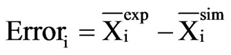 (28)
(28)
3.1. Model 1: Constant Volume and Diffusivity with Equilibrium Boundary Condition
In model 1, the effective mass diffusivity was determined by the optimization algorithm proposed in section 2.5, coupled to the numerical solution presented in section 2. The mass transfer coefficient was kept constant at h = 1 × 10+10 m·s–1, which corresponds to a boundary condition of the first kind. In this case, the objective function has a single minimum, as noted by Silva et al. [21], and the optimization algorithm is not sensitive to the initial value of D. For the experimental data of seedless grape drying, for example, using several significantly different initial values of D, and imposing the relative tolerance of 1 × 10⁻⁴ with 1000 time steps, the optimization delivers the same value for the effective mass diffusivity, as can be seen in Table 1.
Despite of the fact that the last initial value of D is 5 × 10⁵ times greater than the first, the same effective mass diffusivity was obtained in all optimizations. This is consistent with the results of Silva et al. [21], which observed that there is a single value for the diffusivity that minimizes the objective function for the boundary condition of the first kind. The drying simulation considering constant volume and diffusivity for the boundary condition of the first kind is shown in Figure 2.
The statistical indicators of this simulation are: 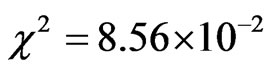 and
and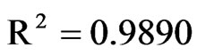 . Using Eq.28, each error can be calculated. The graph of the error distribution is shown in Figure 3, which also shows the possibility to fit a polynomial of degree 5 to the errors.
Figure 3 shows that this model presents a biased fit, with a high value for the average error, once the expected value is zero, and therefore the model should be discarded as an option to describe the drying kinetics of seedless grapes for the experimental conditions investigated in this paper.

Table 1. Effective mass diffusivity obtained through optimization for the boundary condition of the first kind considering constant volume.

Figure 2. Simulation supposing Dirichlet boundary condition, with constant volume and diffusivity (model 1).
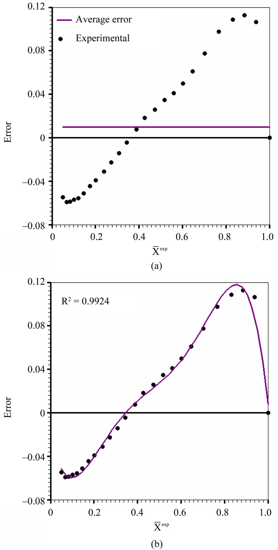
Figure 3. Error distribution for model 1: (a) average error: 9.77 × 10⁻³; (b) fit of a polynomial of degree 5 to the errors: R2 = 0.9924.
3.2. Model 2: Constant Diffusivity, Variable Volume with Equilibrium Boundary Condition
Using the numerical solution presented in this paper and imposing a relative tolerance of 1 × 10⁻⁴ for the convergence of the effective mass diffusivity, with the time of drying divided into 1000 steps,  m2·s–1 is obtained from model 2. A simulation using this value for D results in the graph shown in Figure 4.
The statistical indicators for model 2 are:
 and
and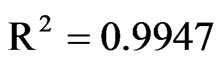 . For this simulation, again using Eq.28, each error can be calculated. The

Figure 4. Simulation for the Dirichlet boundary condition, with variable volume and constant effective diffusivity (model 2).
graph of the error distribution is shown in Figure 5, which also shows the possibility to fit a polynomial of degree 5 to the errors.
Model 2 also delivers a biased fit for the error distribution, with a high value for the average error. Comparison with model 1 indicates that the inclusion of the shrinkage has improved the results, but as can be observed, the equilibrium boundary condition is not really adequate to describe the drying kinetics of seedless grapes for the experimental data analyzed in this article.
3.3. Model 3: Constant Volume and Diffusivity with Convective Boundary Condition
For this model, the analytical solution presented in this paper was explored. In order to guarantee Fo > 0.2, Eq.11 was fitted to the experimental data without the first points, giving B1 = 0.8792, A1 = 9.822 × 10⁻⁶ s–1, and consequently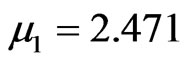 , Bi = 4.115, D = 7.11 × 10⁻¹¹ m2·s–1, h = 4.40 × 10⁻⁸ m·s–1. A graph of this fit is shown in Figure 6(a), while Figure 6(b) shows the drying simulation including all experimental data points.
The error distribution is shown in Figure 7(a), together with the average value of the errors, while Figure 7(b) shows the fit of a polynomial of degree 5 to the errors.
Figure 7 shows that model 3 also yields a biased fit of the error distribution, with a high value for the average error. The advantage of this model is its simplicity, but it does not consider the strong shrinkage of the grapes. In addition, the first experimental points cannot be properly described by the model. On the other hand, the obtained results can be used as initial values for other optimization processes.

Figure 5. Error distribution for model 2: (a) average error: 9.35 × 10⁻³; (b) fit of a polynomial of degree 5 to the errors: R2 = 0.9848.
3.4. Model 4: Constant Diffusivity, Variable Volume with Convective Boundary Condition
An initial value of D which is two or three times greater than the effective mass diffusivity obtained from model 1, generally produces satisfactory results for the simultaneous determination of D and h. This greater initial value of D compensates the resistance to the flux at the boundary.
Although model 1 is not adequate for the description of the drying kinetics of seedless grapes for the experimental conditions investigated in this paper, as discussed

Figure 6. Model 3: (a) fit of Eq.11 to experimental data (Fo > 0.2); (b) Simulation considering all points.
in section 3.1, it can be used for the estimation of an initial value of h by imposing values of the Biot number as 4, 3, 2 or 1 (much lower values than 100, corresponding to the equilibrium boundary condition) in Eq.8. For example, an estimated initial value of D = 5.5 × 10⁻¹¹ m2·s–1 together with an imposed value Bi = 2 leads to an estimation of h = 1.7 × 10⁻⁸ m·s–1 for the initial value of the mass transfer coefficient. Performing the optimization process, with a relative tolerance for the parameters of 1 × 10⁻⁴, and 1000 time steps, the following results are obtained: D = 2.89 × 10⁻¹¹ m2·s–1 and h = 8.05 × 10⁻⁸.
Figure 7. Error distribution for model 3: (a) average error: 1.4970 × 10⁻²; (b) fit of a polynomial of degree 5 to the errors: R2 = 0.9963.
m·s–1, with c2 = 3.848 × 10⁻³ and R2 = 0.9983. These results are much better than those obtained from models 1, 2 and 3. The graph for the moisture content versus time is shown in Figure 8.
The error distribution for model 4 is shown in Figure 9(a), together with the average value of the errors, while Figure 9(b) shows the fit of a polynomial of degree 5 to the errors.
Although model 4 presents better results than models 1, 2 and 3, Figure 9 shows that the average error for this model is large, and the fit still is biased. In fact, the strong shrinkage which occurred during the drying changes the internal structure of the grapes, and this alteration modifies the effective mass diffusivity of the product. Thus,

Figure 8. Simulation for the Cauchy boundary condition, with variable volume and constant effective diffusivity (model 4).
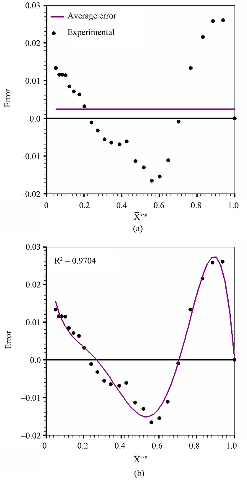
Figure 9. Error distribution for model 4: (a) average error: 2.44 × 10⁻³; (b) fit of a polynomial of degree 5 to the errors: R2 = 0.9704.
models which include a variable effective mass diffusivity should yield better results for the description of the drying kinetics of seedless grapes.
3.5. Model 5: Variable Diffusivity and Volume with Convective Boundary Condition
An inspection of the final part of the graph given in Figure 8 indicates that the value of the effective mass diffusivity should be slightly smaller than the constant value obtained from model 4. This fact suggests that a variable diffusivity can produce better results than a constant value for this parameter. This observation was also made by Silva et al. [28], studying the drying process of bananas. Thus, several optimization processes were accomplished, with the time of drying divided into 2000 steps, supposing different expressions for the effective mass diffusivity D as a function of the local dimensionless moisture content X(r,t). The results obtained for several functions expressing D(X) are summarized in Table 2.
The three expressions of D as a function of X giving the best results are presented in Figure 10. The three functions for the effective mass diffusivity show almost the same behavior for the dimensionless moisture content between 0 and 0.6.
It is interesting to observe in Figure 10 that the functions 1, 2 and 3 are almost constant until the value 0.6 for the local dimensionless moisture content. On the other hand, Figure 11 shows the simulation of the drying kinetic using the function 1 to represent effective mass diffusivity.
For function 1, the effective mass diffusivity varies from 3.04 × 10⁻¹¹ (dimensionless moisture content equal to 0) to 9.36 × 10⁻¹⁰ m2·s–1 (dimensionless moisture content equal to 1), while the convective mass transfer coefficient is 3.56 × 10⁻⁸ m·s–1. For model 5, using function 1, the statistical indicators of the simulation were 
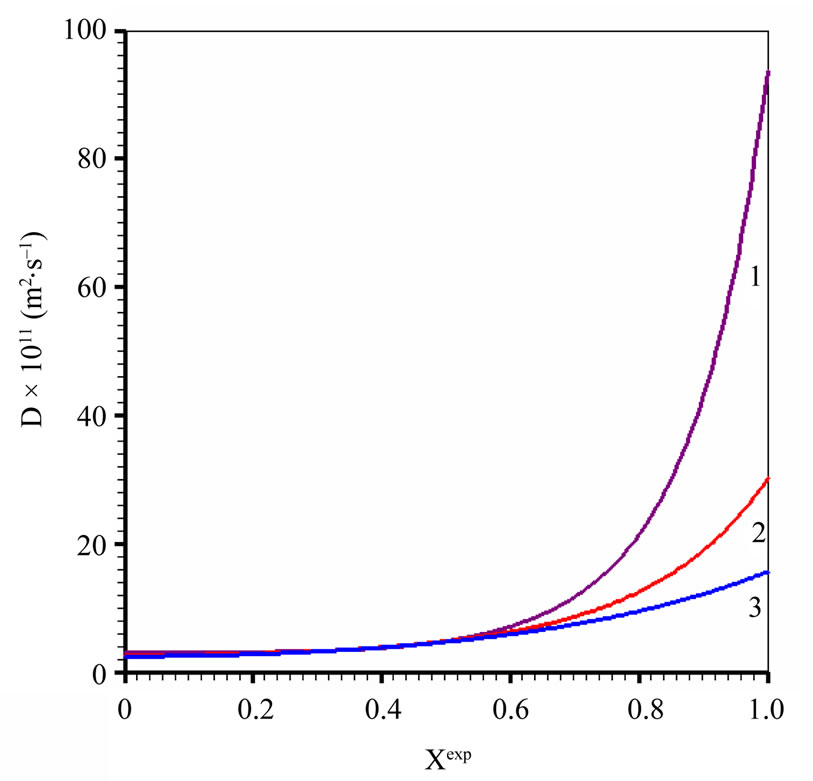
Figure 10. Best functions obtained for the effective mass diffusivity as function of the local dimensionless moisture content (model 5).

Figure 11. Simulation for the Cauchy boundary condition, with variable volume, and the expression for the effective mass diffusivity given by function 1 in Table 2 (model 5).
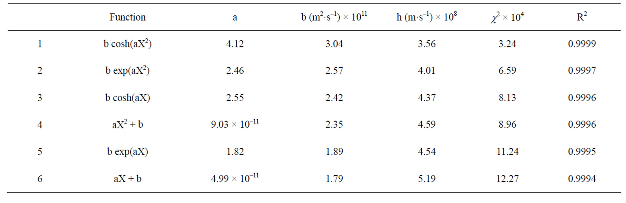
Table 2. Expressions for the effective mass diffusivity as a function of the local dimensionless moisture content considering variable volume.
 and
and . The error distribution is shown in Figure 12.
In Figure 12, it can be observed that the average error is very close to zero; and the error distribution is much less biased than those for the other models. For model 5, the spatial distribution of moisture at specified times can be seen in Figure 13.
Information about the dimensionless moisture content distribution inside the grape is necessary for the description of its drying because it allows analyzing the internal

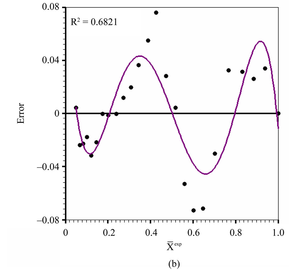
Figure 12. Error distribution for model 5: (a) average error: 2.68 × 10⁻⁵; (b) fit of a polynomial of degree 5 to the errors: R2 = 0.6821.

Figure 13. Contour plots (no scale) showing the radial distribution of moisture at the instants: (a) 13510 s; (b) 26320 s; (c) 41250 s; (d) 59740 s.
stresses during the process. The knowledge of these stresses is important because they may damage the product during the drying process.
4. CONCLUSIONS
An analysis of the all results indicates that the liquid diffusion model well describes drying of seedless grapes, with pretreatment through dipping in hot water, using air in low temperatures.
Models 1 and 2 do not produce good results, indicating that the boundary condition of the first kind should be discarded in a rigorous description of the drying kinetics of seedless grapes under the experimental conditions described in this article.
Although the analytical solution of the diffusion equation with boundary condition of the third kind is an alternative to describe seedless grape drying, such solution does not include the strong effect of the shrinkage. Thus, the third model should also be discarded for the description of the drying kinetics of seedless grapes. Nevertheless, this model can be useful to generate initial values for some optimization process, especially involving numerical solutions.
Model 4 includes the effect of shrinkage, while maintaining the effective mass diffusivity as constant. The results are reasonable, but a closer analysis shows that the effective mass diffusivity should be lower than the obtained value at the final part of the drying process. This suggests that the change of the internal structure caused by shrinkage also affects the effective mass diffusivity.
A better model for the description of seedless grape drying, with pretreatment through dipping in hot water, must include: 1) shrinkage, 2) convective boundary condition, and 3) variable effective mass diffusivity. The best result was obtained supposing an expression for the effective mass diffusivity, which increases with the local dimensionless moisture content. For the analyzed experimental data, the effective mass diffusivity is best represented by function 1 given in Table 2. In this case, the statistical indicators of the simulation can be considered excellent.
In order to compare the results, the model 5 characterized in the last paragraph provides a chi-square which is about 264 times smaller than the chi-square obtained for the model 1. in addition the error distribution for model 5 can be considered random.
REFERENCES
- Margaris, D.P. and Ghiaus, A.G. (2007) Experimental study of hot air dehydration of Sultana grapes. Journal of Food Engineering, 79, 1115-1121. doi:10.1016/j.jfoodeng.2006.03.024
- Pangavhane, D.R., Sawhney, R.L. and Sarsavadia, P.N. (1999) Effect of various dipping pretreatment on drying kinetics of Thompson seedless grapes. Journal of Food Engineering, 39, 211-216. doi:10.1016/S0260-8774(98)00168-X
- Azzouz, S., Guizani, A., Jomaa, W. and Belghith, A. (2002) Moisture diffusivity and drying kinetic equation of convective drying of grapes. Journal of Food Engineering, 55, 323-330. doi:10.1016/S0260-8774(02)00109-7
- Doymaz, I. and Pala, M. (2002) The effects of dipping pretreatments on air-drying rates of the seedless grapes. Journal of Food Engineering, 52, 413-417. doi:10.1016/S0260-8774(01)00133-9
- Doymaz, I. (2006) Drying kinetics of black grapes treated with different solutions. Journal of Food Engineering, 76, 212-217. doi:10.1016/j.jfoodeng.2005.05.009
- Esmaiili, M., Rezazadeh, G., Sotudeh-Gharebagh, R. and Tahmasebi, A. (2007) Modeling of the seedless grape drying process using the generalized differential quadrature method. Chemical Engineering and Technology, 30, 168-175. doi:10.1002/ceat.200600151
- Di Matteo, M., Cinquanta, L., Galiero, G. and Crescitelli, S. (2000) Effect of a novel physical pretreatment process on the drying kinetics of seedless grapes. Journal of Food Engineering, 46, 83-89. doi:10.1016/S0260-8774(00)00071-6
- Ramos, I.N., Miranda, J.M.R., Brandão, T.R.S. and Silva, C.L.M. (2010) Estimation of water diffusivity parameters on grape dynamic drying. Journal of Food Engineering, 97, 519-525. doi:10.1016/j.jfoodeng.2009.11.011
- Bennamoun, L. and Belhamri, A. (2006) Numerical simulation of drying under variable external conditions: Application to solar drying of seedless grapes. Journal of Food Engineering, 76, 179-187. doi:10.1016/j.jfoodeng.2005.05.005
- Hacihafizoglu, O., Cihan, A., Kahveci, K. and Lima, A.G.B. (2008) A liquid diffusion model for thin-layer drying of rough rice. European Food Research and Technology, 226, 787-793. doi:10.1007/s00217-007-0593-0
- Silva, W.P., Precker, J.W., Silva, C.M.D.P.S. and Gomes, J.P. (2010) Determination of effective diffusivity and convective mass transfer coefficient for cylindrical solids via analytical solution and inverse method: Application to the drying of rough rice. Journal of Food Engineering, 98, 302-308. doi:10.1016/j.jfoodeng.2009.12.029
- Queiroz, M.R. and Nebra, S.A. (2001) Theoretical and experimental analysis of the drying kinetics of bananas. Journal of Food Engineering, 4, 127-132. doi:10.1016/S0260-8774(00)00108-4
- Zhan, J.-f., Gu, J.-y. and Cai, Y.-c. (2007) Analysis of moisture diffusivity of larch timber during convective drying condition by using Crank’s method and Dincer’s method. Journal of Forestry Research, 18, 199-203. doi:10.1007/s11676-007-0040-x
- Kaya, A., Aydın, O. and Dincer, I. (2010) Comparison of experimental data with results of some drying models for regularly shaped products. Heat Mass Transfer, 46, 555- 562. doi:10.1007/s00231-010-0600-z
- Jia, C., Yang, W., Siebenmorgen, T.J. and Cnossen, A.G. (2001) Development of computer simulation software for single grain kernel drying, tempering and stress analysis. transactions of the ASAE, 45, 1485-1492.
- Gastón, A.L., Abalone, R.M. and Giner, S.A. (2002) Wheat drying kinetics. Diffusivities for sphere and ellipsoid by finite elements. Journal of Food Engineering, 52, 313-322. doi:10.1016/S0260-8774(01)00121-2
- Li, Z., Kobayashi, N. and Hasatani, M. (2004) Modelling of diffusion in ellipsoidal solids: a comparative study. Drying Technology, 22, 649-675. doi:10.1081/DRT-120034256
- Wu, B., Yang, W. and Jia, C. (2004) A three-dimensional numerical simulation of transient heat and mass transfer inside a single rice kernel during the drying process. Biosystems Engineering, 87, 191-200. doi:10.1016/j.biosystemseng.2003.09.004
- Carmo, J.E.F. and Lima, A.G.B. (2005) Drying of lentil including shrinkage: a numerical simulation. Drying Technology, 23, 1977-1992. doi:10.1080/07373930500210424
- Silva, W.P., Silva, C.M.D.P.S., Silva, D.D.P.S. and Silva, C.D.P.S. (2008) Numerical Simulation of the Water Diffusion in Cylindrical Solids. International Journal of Food Engineering, 4, 1-16. doi:10.2202/1556-3758.1394
- Silva, W.P., Precker, J.W., Silva, C.M.D.P.S. and Silva, D.D.P.S. (2009) Determination of the effective diffusivity via minimization of the objective function by scanning: application to drying of cowpea. Journal of Food Engineering, 95, 298-304. doi:10.1016/j.jfoodeng.2009.05.008
- Silva, W.P., Silva, C.M.D.P.S., Farias, V.S.O. and Silva, D.D.P.S. (2010) Calculation of the convective heat transfer coefficient and cooling kinetics of an individual fig fruit. Heat and Mass Transfer, 46, 371-380. doi:10.1007/s00231-010-0577-7
- Luikov, A.V. (1968) Analytical heat diffusion theory. Academic Press Inc. Ltd., London.
- Crank, J. (1992) The mathematics of diffusion. Clarendon Press, Oxford.
- Patankar, S.V. (1980) Numerical heat transfer and fluid flow. Hemisphere Publishing Corporation. New York.
- Bevington, P.R. and Robinson, D.K. (1992) Data reduction and error analysis for the physical sciences. 2nd edition, WCB/McGraw-Hill, Boston.
- Taylor, J.R. (1997) An introduction to error analysis. 2nd Edition, University Science Books, Sausalito.
- Silva, W.P., Silva, C.M.D.P. S., Farias, V.S.O. and Gomes, J.P. (2012) Diffusion models to describe the drying process of peeled bananas: optimization and simulation. Drying Technology, 30,164-174. doi:10.1080/07373937.2011.628554