International Journal of Geosciences
Vol.4 No.2(2013), Article ID:29377,11 pages DOI:10.4236/ijg.2013.42038
Modeling an Oil Spill along the Southern Brazilian Shelf: Forcing Characterization and Its Influence on the Oil Fate
1Instituto de Oceanografia, Universidade Federal do Rio Grande, Rio Grande, Brazil
2Instituto de Matemática, Estatística e Física, Universidade Federal do Rio Grande, Rio Grande, Brazil
3Centro de Ciência Computacionais, Universidade Federal do Rio Grande, Rio Grande, Brazil
Email: caiodalaqua@hotmail.com
Received December 19, 2012; revised January 17, 2013; accepted February 16, 2013
Keywords: Oil Spill Model; Wind Driven Circulation; Weathering
ABSTRACT
Oil spills can generate multiple effects in different time scales on the marine ecosystem. The numerical modeling of these processes is an important tool with low computational cost which provides a powerful appliance to environmental agencies regarding the risk management. In this way, the objective of this work is to evaluate the influence of a number of physical forcing acting over a hypothetical oil spill along the Southern Brazilian Shelf. The numerical simulation was carried out using the ECOS model (Easy Coupling Oil System), an oil spill model developed at the Universidade Federal do Rio Grande—FURG, coupled with the tridimensional hydrodynamic model TELEMAC3D (EDF, France). The hydrodynamic model provides the current velocity, salinity and temperature fields used by the oil spill model to evaluate the behavior and the fate of the spilled oil. The results suggest that the local wind influence is the main forcing driven the fate of the spilled oil, and this forcing responds for more than 60% of the oil slick variability. The direction and intensity of the costal currents control between 20% and 40% of the oil variability, and the currents are important controlling the behavior and the tridimensional transportation of the oil. On the other hand, the turbulent diffusion is important for the horizontal drift of the oil. The weathering results indicate 40% of evaporation and 80% of emulsification, and the combination of these processes leads an increasing of the oil density around, 53.4 kg/m³ after 5 days of simulation.
1. Introduction
The outpouring of oil and derivatives on the marine ecosystem is an important subject to be considered by the modern society, since the oil is composed by toxic substances that exposed on the environment can create chronic effects [1]. In this way, the efficient recovering of the affected region can take dozens to hundreds years, or even be irreversible, affecting the society in different ways. According to [2], half of the world oil production is transported by the oceans, meaning 31.5 billion gallons. The oil entrance on the marine environment varies from 1.7 to 8.8 million tons/year, where the marine transportation is responsible for 23.5% of this total, while much concerns in regular ship operations, and a small part (about 10%) represent the accidental spills [3]. According to [4], the routine operations in harbors, accidents in transport terminal networks and urban effluents have been the major oil sources for the ocean.
The Southern Brazilian Shelf (Figures 1(a) and (b)) presents high susceptibility for eventual accidents regarding the oil spill, since nowadays there is an intense oil transportation in this region due to the Rio Grande Harbor, the Transpetro Waterway Terminal (Petrobras) and the Riograndense Oil Refinery S/A. The major part of the transportation activities identified in this region occurs on the estuarine environment of the Patos Lagoon and near the adjacent coastal region. In 2003 year almost 3000 ships were moved and in during 2008 year more than 60,000 tons of oil was transported in the Rio Grande Harbor (www.portoriogrande.com.br).
The oil spill in estuaries is worrying because these are ecological and economically important environments. The estuaries retain a large amount of the spilled oil, increasing the contamination effects. Therefore, the estuaries are the environments that present the major sensibility degree according with the scales used in the oil sensitivity maps.
According to the Brazilian legislation, the numerical simulations of spilled oil must define the area of indirect influence of this activity, in which all the environment diagnostic is based. In this sense, the diagnostic defines and simulates scenarios allowing the development of
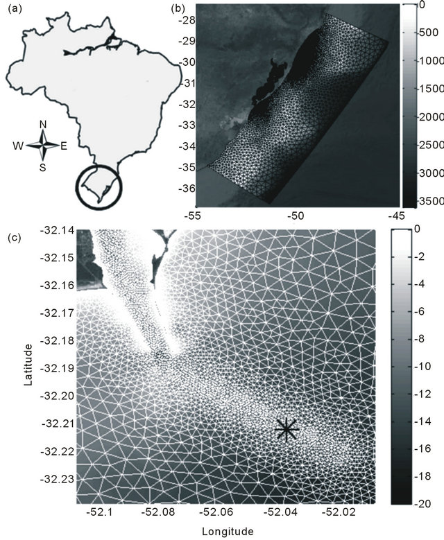
Figure 1. Study region. (a) The numerical domain; and (b) The zoom in the region of the oil spill; (c) The color bar indicates the bathymetric variability and the position of the oil spill is represented by the black cross.
strategies for an oil spill accident in the ocean into the emergency plane of the companies. Therefore, the objective of this paper is to investigate the effects of different physical forcing controlling the behavior and the fate of an oil spill near the Patos Lagoon entrance.
2. Hydrodynamic Model
The numerical model TELEMAC3D (EDF—Laboratoire National d’ Hydraulique et Environnement of the Company Eletrecité de France) has been used for tridimensional hydrodynamic simulations. This model solves the Navier-Stokes equations using finite element techniques for spatial discretization. It considers the free surface variation for incompressible fluids and considers the Boussinesq approximation in order to solve the momentum equations [5]. A detailed discussion regarding the TELEMAC3D, the calibration and validation tests for hydrodynamics and morphodynamics along the Southern Brazilian Shelf can be found in [6-9].
3. The ECOS Model
The ECOS (Easy Coupling Oil Model) has been developed through techniques of modular programming between object-oriented paradigm, which allows a better structuring and control of the libraries related to the subprograms and functions. This type of organization allows the compilation of each module apart, saving computational time, so that the reutilization of the functions is facilitated. The model uses a coupling interface, which contains all the necessary information to be shared by the oil and hydrodynamic model. The processes of what the oil is subject when arrives at the environment, such as spreading, turbulent diffusion, evaporation, dispersion and emulsification are implemented.
4. Mathematical Description of the Oil Transport and Weathering
This section quickly describes the mathematical formulations used by some actual oil models and those used by the ECOS model developed at FURG. This model treats the oil like discrete particles using Lagrangian approximation to evaluate the tracer (particles) proprieties during time.
The tracer trajectory is evaluated considering the oil like a large number of particles which moves independently in water. The tracer velocities are interpolated from the current velocity in each node of the hydrodynamic numerical domain (Figure 1(b) and Figure 2).
The final tracer position depends on four different factors: 1) Current velocity; 2) Wind velocity; 3) Spreading effect; and 4) Turbulent diffusion. In this work, the effects associated with the slick drift are described in the following sections. Figure 3 shows all the processes acting in an oil spill at the marine environment.
4.1. Advection
In this work, all the effects which are independent from the physical-chemical effects are considered like advective forcing. In these classes are evaluated the drifting driven by the current and winds, and also the vertical transport due to the buoyancy associated with the difference of density between the oil and the water. The zonal (U), meridional (V) and vertical (W) components of the velocity are calculated by the Equations (1)-(3), respectively. Where and
and  are the coefficients of influence of the currents and winds.
 (1)
(1)
 (2)
(2)
 (3)
(3)
The particle buoyancy law (Equation (4)) is based on a modified stokes law for the oil according to [11,12]. In
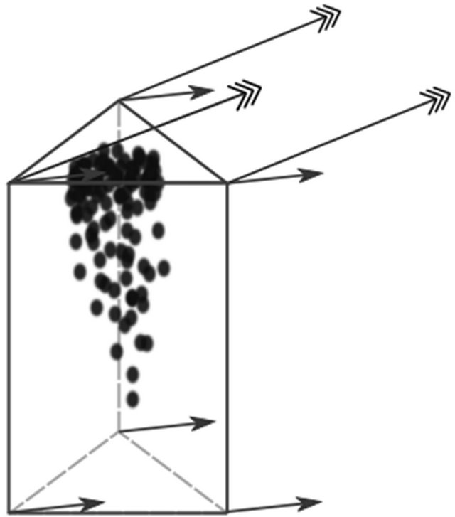
Figure 2. Advective forces in a prismatic element. Triple arrows indicate the wind contribution and the single arrows indicate the current contribution. The trajectory of each particle is an algebraic interpolation of these components.

Figure 3. Oil weathering processes in marine environments [10].
this formulation  is the vertical particle velocity.
 (4)
(4)
where: g is the gravity acceleration, ρo is the oil density at the initial time to, ρw is the average salt water density and νw is the water viscosity.
Maximum and minimum droplets sizes are evaluated through [13] formulations (Equations (5) and (6)). Thus, the mean droplet size is an arithmetic mean of the maximum and minimum droplets size (Equation (7)).
 (5)
(5)
 (6)
(6)
 (7)
(7)
This formulation uses wave energy (σ) and wave period (ω), at this moment the model uses constants averaged values for this parameters.
4.2. Diffusion
All the processes that depend on the oil physical-chemical characteristics are considered as diffusion processes. This class fits spreading and turbulent diffusion, and both processes are function of the tensions in the oil-water interface. In this way, these processes are represented through “random-walk” techniques.
4.2.1. Spreading
The spreading is a horizontal expansion effect due to the different superficial tensions between the water and the oil. This represents a force balance between gravity acceleration, inertia, viscous and superficial tensions. This process is very important during initial moments after spill.
The algorithm used to evaluate the oil spreading determines the random velocities Ud and Vd uniform distribution in the range [−Ur + Ur] and [−Vr + Vr] (along x and y directions, respectively) proportional to the diffusion coefficients, which are calculated assuming that the Lagrangian tracers spread according with the solution proposed by [14]. The relationship between the diffusion coefficients Dx and Dy and the interval of the flotation velocity [−Ur + Ur] and [−Vr + Vr] are adopted according to [14]. The diffusion coefficients Dx and Dy are calculated according to Equation (8):
 (8)
(8)
The intervals of flotation [−Ur + Ur] and [−Vr + Vr] are calculated according to Equations (9) and (10).
 (9)
(9)
 (10)
(10)
The random velocities Usi and Vsi are, therefore, determined by the formulation proposed by [15] in Equations (11) and (12).
 (11)
(11)
 (12)
(12)
where R1 and R2 are random numbers generated from a normal distribution between 0 and 1.
4.2.2. Turbulent Diffusion
The horizontal turbulent diffusion is evaluated through a modified mixing length turbulence model for the oil spills. Maximum distance that a particle can go from actual (t) position is calculated in Equation (13), equivalent to a traditional mixing length model. Equations (14) and (15) estimate the particle velocities based in a “random walk” method.
 (13)
(13)
 (14)
(14)
 (15)
(15)
4.3. Particle Path Finally, after the definition of all forces acting in a particle, the positions can be integrated in time, by an Euler forward method. Equations (16)-(18) evaluate each particle position during time.
 (16)
(16)
 (17)
(17)
 (18)
(18)
4.4. Evaporation
Evaporation is considered one of the most important processes in an oil spill, once it controls the mass balance and can cause about 75% of lost mass according to [16]. Evaporation processes are linked to the wind velocity and the spill area. The evaporation rates are determined according to [17] by Equation (19).
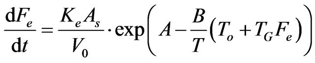 (19)
(19)
4.5. Emulsification
The creation of a mousse, mainly characteristic of this process, occurs due to the incorporation of water in oil slick through the polar components of the oil. Equation (20) represents the water incorporation in oil according to [18].
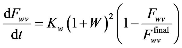 (20)
(20)
4.6. Oil Density
This process is very important in the oil spill modeling, once the buoyancy of the oil particles is determined. It causes the sinking of the oil if the water density is lower than the oil density. In a quickly view, during the evaporation process occurs mass lost, while during the emulsification process occurs mass gain of the oil slick. Therefore, the balance of these processes defines the final oil density. Equation (21) evaluates the oil density according to [19].
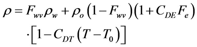 (21)
(21)
5. Coupling between the Models
The ECOS model has been directly coupled to the TELEMAC3D source code (see [20]). In TELEMAC3D, the hydrodynamics and the winds are used by the Lagrangian module for the oil model to evaluate the tracer positions at each time step. The salinity, temperature, and the density of the water, from TELEMAC3D, are transferred by the weathering module, which evaluates the oil evaporation, emulsification and density. Figure 4 shows the coupling between these models.
Boundary Conditions
Time series of oceanographic data are used as boundary conditions. The boundary conditions currently implemented include time series of river discharge, water levels, salinity, temperature, current and wind velocity. The river discharge was obtained by ANA (Agência Nacional de Águas) website. Salinity, temperature, current velocity and water levels were obtained by the global predict model OCCAM (Ocean Circulation and Climate Advanced Model). Wind and air temperature data were provided for the NOAA page (National Oceanic & Atmospheric Administration).
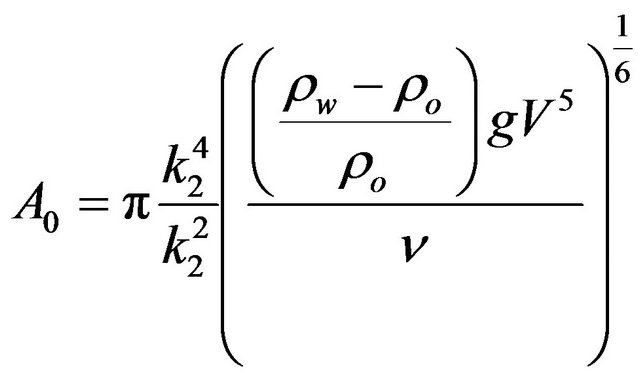
6. Initial Conditions and Oil Properties
Nowadays, the oil model considers an accidental punctual spill (see Figure 1(b)), with a circular form which can be estimated by [21] formulations. Once the initial gravitational-inertial phase is extremely quick, the spilled initial

Figure 4. Information flux between the TELEMAC3D and the ECOS model.
 (22)
(22)
In this work, the initial conditions of the oil model are:

area is defined at the end of this phase with the beginning of the gravitational-viscous phase in Equation (22).
7. Results and Discussion
In order to accomplish the objectives, two simulations were carried out. The first simulation (simulation 1) includes all the physical forcing the oil slick dynamics. On the other hand, the second simulation (simulation 2) was carried out without consideration of the local wind influence acting over the oil slick. The results regarding only the hydrodynamic processes are not analyzed in this work, because an extensive description of hydrodynamic processes along the Southern Brazilian Shelf can be found in: [20,22] and [6-9].
7.1. Simulation 1
Results for the temporal evolution of the tracers are presented in Figure 5 (Salinity is represented by the grayish scale). After the spill occurs a quickly initial horizontal expansion due to the spreading effect and the horizontal turbulence. The local wind over the oil slick controls the behavior and the final fate of those tracers but past 30 hours of simulation the oil slick reaches the coastline.
Through the analysis of the wind direction in Figure 6, it becomes clear that south quadrant winds are dominant in the first 20 hours of simulation followed afterwards by north quadrant winds in the last hours. The south quadrant winds are downwelling favorable along the Southern Brazilian Shelf and this effect is observed on the oil slick behavior during the spreading towards the coastline. The behavior observed by the oil slick is very similar to the Patos Lagoon coastal plume studied by [6-9].
7.2. Simulation 2
Results without the local wind influence acting over the oil slick are presented in Figure 7. The initial steps of the simulation are quite similar to the simulation considering all forcing together, with dominance of the diffusive processes. However the oil slick never reaches the coastline during 5 days of simulation, because the influence of the local wind effect is not considered.
 (a)
(a)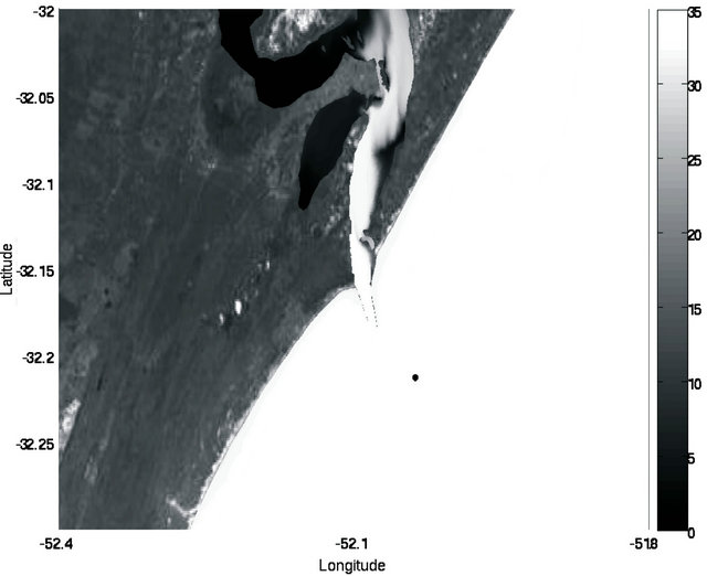 (b)
(b) (c)
(c)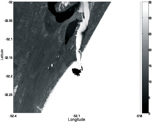 (d)
(d)
Figure 5. Evolution of the oil trajectory following intervals of 10 hours. Initial instant (a), after 10 hours (b), after 20 hours (c) and after 30 hours (d) of simulation.
 (a)
(a) (b)
(b)
Figure 6. Time series of the intensity and direction of winds during the whole period. The first 30 hours after the oil spill (a) and 120 hours during the oil spill simulation (b).
The oil slick behavior and its further destination are strongly influenced by the coastal wind driven circulation pattern with the alongshore drifting to the south region due to northeastern winds. This behavior is consistent with results obtained by [6-9] among others, for the coastal circulation near the Patos Lagoon entrance.
7.3. Analysis of the Physical Forcing
In order to quantify the contribution of the local wind effect as determinant factor controlling the oil slick behavior, a time series analysis is presented. Figure 8 shows the non dimensional contribution of all the physical forcing acting on the oil slick during the period of simulation (120 hours). The non dimensional contribution is obtained through the ratio between each component (wind, currents, turbulence and spreading) and all the contributions controlling the oil slick behavior. The results suggest that the wind effects appear as the most important contribution, responding for more than 60% of variability during almost all the time, except in the first hours when the currents dominate the spreading of the spilled oil.
The second major contribution, controlling from 20% to 40% of variability, is provided by the coastal currents which drives the oil initially on the direction of the superficial currents, except by the particles that suffer process of sinking according with the following tridimensional circulation pattern developed. The turbulent forces act in a secondary way responding for less than 20% of variability generating a horizontal disintegration of the oil slick during all the period of simulation. The spreading component decreases very fast, being active on the first hours of simulation. However, this component dominates the initial disintegration of the slick.
During the first 2 hours of simulation, the currents dominate the spreading of the oil spill because of the time response associated with the local wind influence acting over the oil slick. In addition, during periods of changing in wind direction (about 10 hours of simulation), the costal currents turn to dominate the behavior of the oil slick.
The direct correlation between the displacement of the oil slick and the local wind influence is observed and the most important cycles occur from 12 to 16 hours, following the short time variability of the winds over the study region. The spectral content and the correlation between these time series (Figure 9(a)) were investigated using cross-wavelet analysis. This method locates power variations within the discrete time series over a range of scales and provides the local power spectrum.
The analysis of the local power spectrum (Figure 9(b)) corroborated that the physical processes between 12 and 16 hours were the main mechanisms controlling the oil slick behaviour along the inner continental shelf. According with the wavelet analysis, the events controlling the fate of the oil slick present a well-defined pattern associated to the sea breeze occurring throughout the whole period.
 (a)
(a) (b)
(b)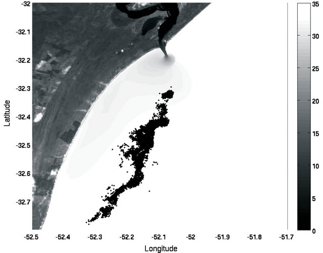 (c)
(c)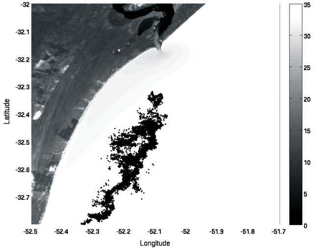 (d)
(d)
Figure 7. Evolution of the oil trajectory following intervals of 10 hours. Initial instant (a), after 10 hours (b), after 20 hours (c) and after 30 hours (d) of simulation.

Figure 8. Non-dimensional contribution of the physical forcing during the simulated period.
 (a)
(a)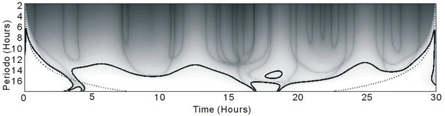 (b)
(b)
Figure 9. Time series of the physical contributions and wind intensity: (a) The local power spectrum through the cross-wavelet analysis using the Morlet wavelet; (b) Thick contour lines enclose regions of greater than 95% confidence for a red-noise process with a lag-1 coefficient of 0.2. Cross-hatched regions indicate the cone of influence where edge effects become important.
7.4. Weathering Properties
On the analysis of the tracer trajectory there is not enough information to explain the oil spill behavior. Therefore, it is necessary to consider the analysis of the scalar properties, such as evaporation and emulsification that act directly on the oil density.
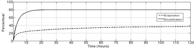
Figure 10 shows the temporal evolution of the scalar properties calculated by the oil model. It is possible to observe that a great amount of the oil evaporates (around 40%) and emulsifies (around 70%) during the first 48 hours of simulation. The combination of the emulsification and evaporation effects cause some increase in the oil density.
The behavior of the emulsification is corroborated by the experiments proposed by [23] that analyzing emulsions series showed that the curve follows an exponential pattern with a quick incorporation of water during the first 24 hours. The evaporation behavior is consistent with the results observed in [11] and by the model ADIOS2 [24].
The increase of the oil density makes it reach a density very close to the salt water, which causes a balance of phases enhancing the importance of the effects controlled by the tridimensional circulation causing processes such as vertical dissolution and sedimentation of the spilled oil.
8. Final Considerations
The principal conclusions obtained in this study are:
• Wind acting over the oil slick is the most important forcing controlling its behavior and further destination. This forcing mechanism responds for more than 60% of the oil variability during almost all the time.
• The winds from the Southern (Northern) quadrant induce the movement of the oil slick directly to the coast (offshore).
• Intensity and direction of the coastal currents control between 20% and 40% of the oil variability during the simulated period. This forcing is important for the vertical distribution of the oil along the water column. The diffusive forcing represents less than 20% of the variability and it has secondary effect acting mainly on the horizontal dispersion of the oil slick.
• During 120 hours of simulation about 40% of the oil evaporates and 80% of the oil emulsifies. The combination of these effects generates an increase of 53.4 kg/m3 on the density, showing the magnitude of the mixture and the aging processes.
• Simulation without the consideration of the winds on the oil slick is slacking realistic because the oil slick does not reach the coast any moment even by the influence of favorable winds. Besides, after 48 hours of simulation, the aging processes are dominant and, in some way, it commits the results obtained by the spreading of the oil slick after this period.
9. Acknowledgements
The authors thank to the Conselho Nacional de Desenvolvimento Científico e Tecnológico—CNPQ and the Agência Nacional do Petróleo—ANP for the fellowships
 (a)
(a)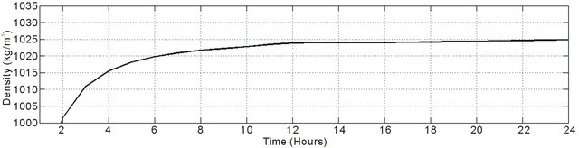 (b)
(b)
Figure 10. Time series for the scalar properties of the oil. Emulsification and evaporation (a) and density (b) time series.
provided which helped the development of this work. The authors still thank to the Fundação de Amparo à Pesquisa do Estado do Rio Grande do Sul—FAPERGS for partially support this work (Process: 11/1767-4, Process: 1018144 and Process: 179912-3). Further acknowledgements go to the Brazilian Navy for providing detailed bathymetric data for the coastal area, to the Brazilian National Water Agency (ANA) and the National Oceanic & Atmospheric Administration (NOAA) for supplying the fluvial discharge and wind data sets, respectively, and to the EDF for providing the TELEMAC System to accomplish this research.
REFERENCES
- K. A. Burns, S. Garrity, D. Jorissen, J. Macpherson, M. Stoelting, J. Tierney and L. Y. Simmons, “The Galeta Oil Spill ii. Unexpected Persistence of Oil Trapped in Mangrove Sediments Morlaix Twenty Years after the Amoco Cadiz Oil Spill,” Estuarine, Coastal and Shelf Research, Vol. 38, No. 4, 1994, pp. 349-364. doi:10.1006/ecss.1994.1025
- R. B. Clark, “Marine Pollution,” Oxford University Press, Oxford, 2001.
- R. Fernandes, “Modelação de Derrames de Hidrocarbonetos. Dissertção de Mestrado,” Instituto Superior Técnico—Universidade de Lisboa, 2001.
- R. C. Pereira and A. Soares-Gomes, “Biologia Marinha,” Inferência, Rio de janeiro, 2002, pp. 318-319.
- J. M. Hervouet, “Free Surface Flows: Modelling with Finite Element Methods,” John Wiley & Sons, Hoboken, 2007.
- W. C. Marques, E. Fernandes, I. Monteiro and O. O. Möller, “Numerical Modeling of the Patos Lagoon Coastal Plume, Brazil,” Continental Shelf Research, Vol. 29, No. 3, 2000, pp. 556-571. doi:10.1016/j.csr.2008.09.022
- W. C. Marques, E. Fernandes and O. O. Möller, “Straining and Advection Contributions to the Mixing Process of the Patos Lagoon Coastal Plume, Brazil,” Journal of Geophysical Research, Vol. 115, No. C6, 2010, pp. 1-23. doi:10.1029/2009JC005653
- W. C. Marques, E. Fernandes and A. Malcherek, “Dynamics of the Patos Lagoon Coastal Plume and Its Contribution to the Deposition Pattern of the Southern Brazilian Inner Shelf,” Journal of Geophysical Research, Vol. 115, No. C10, 2010, pp. 1-22. doi:10.1029/2010JC006190
- W. C. Marques, E. Fernandes, A. L. A. O. Rocha and A. Malcherek, “Energy Converting Structures in the Southern Brazilian Shelf: Energy Conversion and Its Influence on the Hydrodynamic and Morphodynamic Processes,” Sciences, Vol. 1, No. 1, 2012, pp. 61-85.
- M. Bollmann, “World Ocean Review,” Maribus, 2010.
- D. P. French-Mccay, “Oil Spill Impact Modeling: Development and Validation,” Environmental Toxicology and Chemistry, Vol. 23, No. 10, 2004, pp. 2441-2456.
- X. Chao, N. J. Shankar and H. F. Cheong, “Twoand Three-Dimensional Oil Spill Model for Coastal Waters,” Ocean Engineering, Vol. 28, No. 12, 2001, pp. 1557- 1573. doi:10.1016/S0029-8018(01)00027-0
- A. H. Al-Rabeh, H. M. Cekirge and N. Gunay, “A Stochastic Simulation Model of Oil Spill Fate and Transport,” Applied Mathematical Modelling, Vol. 13, No. 6, 1989, pp. 322-329. doi:10.1016/0307-904X(89)90134-0
- P. Leitão, “Modelo de Dispersão Lagrangeano Tridimensional—Dissertação de Mestrado,” Universidade Técnica de Lisboa, Lisboa, 1996.
- R. Proctor, R. A. Flather and A. J. Elliot, “Modelling Tides and Surface Drift in the Arabian Gulf—Application to the Gulf Oil Spill,” Continental Shelf Research, Vol. 14, No. 5, 1994, pp. 531-545. doi:10.1016/0278-4343(94)90102-3
- M. Fingas, “The Evaporation of Oil Spills: Development and Implementation of New Prediction Methodology,” Marine Environmental Modelling Seminar, Vol. 98, Lillehammer, Norway, 1998.
- W. Stiver and D. Mackay, “Evaporation Rate of Spills of Hydrocarbons and Petroleum Mixtures,” Environmental Science and Technology, Vol. 18, No. 11, 1984, pp. 834- 840. doi:10.1021/es00129a006
- D. Mackay, I. A. Buistt, R. Mascarenhas and S. Paterson, “Oil Spill Processes and Models,” Environment Canada, Ottawa, 1980.
- I. Buchanan and N. Hurford, “Methods for Predicting the Physical Changes in Oil Spilt at Sea,” Oil & Chemical Pollution, Vol. 4, No. 4, 1988, pp. 311-328. doi:10.1016/S0269-8579(88)80004-2
- L. F. Mello, C. E. Stringari, R. T. Eidt and W. C. Marques, “Desenvolvimento de Modelo Lagrangiano de Transporte de Óleo: Estruturação e Acoplamento ao Modelo Hidrodinâmico TELEMAC3D,” Pesquisas Aplicadas em Modelagem Matemática, Vol. 1, No. 1, 2012, pp. 1-21.
- J. A. Fay, “The Spread of Oil Slicks on a Calm Sea,” In: D. P. Hoult, Ed., Oil on the Sea, Plenum Press, New York, 1969, pp. 53-63.
- C. E. Stringari, L. F. Mello, R. T. Eidt and W. C. Marques, “Estudo Numérico Lagrangiano Para Derrames de Óleo na Região Oceânica Adjacente ao Porto de Rio Grande—RS,” Conferência Internacional em Tecnologias Naval e Offshore: Ciência e Inovação, Rio Grande, 2012, p. 4.
- H. Wang and C. P. Huang, “The Effect of Turbulence on Oil Emulsification,” Workshop on Physical Behavior of Oil in the Marine Environment, 1979.
- NOAA, “ADIOS (Automated Data Inquiry for Oil Spills) Version 2.0,” Hazardous Materials Response and Assessment Division, NOAA, The US Coast Guard Research and Development Center, Seattle, 2000.