International Journal of Geosciences
Vol.3 No.5(2012), Article ID:25005,10 pages DOI:10.4236/ijg.2012.35114
Remote Sensing, Model-Derived and Ground Measurements of Snow Water Equivalent and Snow Density in Alaska
Geophysical Institute, University of Alaska Fairbanks, Fairbanks, USA
Email: reginald.muskett@gmail.com
Received September 1, 2012; revised October 1, 2012; accepted October 31, 2012
Keywords: AMSR-E; GlobSnow; GIPL Model; Ground Measurements; Snow Water Equivalent; Snow Density; Alaska
ABSTRACT
Snow water equivalent (SWE) is important for investigations of annual to decadal-scale changes in Arctic environment and energy-water cycles. Passive microwave satellite-based retrieval algorithm estimates of SWE now span more than three decades. SWE retrievals by the Advanced Microwave Scanning Radiometer for the Earth Observation System (AMSR-E) onboard the NASA-Aqua satellite ended at[RM1] October 2011. A critical parameter in the AMSR-E retrieval algorithm is snow density assumed from surveys in Canada and Russia from 1940s-1990s. We compare ground SWE measurements in Alaska to those of AMSR-E, European Space Agency GlobSnow, and GIPL model. AMSR-E SWE underperforms (is less than on average) ground SWE measurements in Alaska through 2011. Snow density measurements along the Alaska permafrost transect in April 2009 and 2010 show a significant latitude-gradient in snow density increasing to the Arctic coast at Prudhoe Bay. Large[RM2] differences are apparent in comparisons of our measured mean snow densities on a same snow cover class basis March-April 2009-2011 Alaska to those measured in Alaska winter 1989-1992 and Canadian March-April 1961-1990. Snow density like other properties of snow is an indicator of climate and a non-stationary variable of SWE.
1. Introduction
Snow water equivalent (SWE), the equivalent amount of water of a snow on the ground is a fundamental parameter of climate, environment and energy-water cycles on Earth. SWE is the uniform thickness of water melted from snow in length units of meters (m), snow depth multiplied by snow density is[RM3] divided by pure-water density) or in mass/volume units of kilograms/meter-cubed (kg/m2), snow depth multiplied by snow density). In this report we use the length scale centimeter for SWE and the mass/volume scale g/cm3 for snow density.
Properties of perennial and seasonal snow such as density, microstructure and layering are spatially and temporally heterogeneous on scales of 103 to 105 m [1]. Snow density, i.e. bulk snow density, (Table 1) is influenced by temperature changes, grain size and microstructure, granular humidity and surface wind after deposition [2]. This dependence is due to the low pressuretemperature triple-point thermodynamics of ice [3]. Due to compaction and metamorphic processes within snowpack, snow density changes during the winter season.
Ernst Gorge was one of the first to investigate densification of snow on high polar glaciers at Eismitte station during Wegener’s Greenland expedition 1930-1931 [4].
Our investigation focuses on comparisons of seasonal SWE derived by passive microwave satellite sensor, assimilated and modeled to ground measurements from March 2004 through March 2011. The comparisons are point-wise on a same-day-month and same-datum basis in Alaska (Figure 1). The geographic distributions of the ground measurement locations make them suitable for comparison with satellite-sensor and model derived SWE. Our works include comparisons of mean snow densities (mean bulk snow densities) measured at locations along the Alaska permafrost transect from central Alaska to Prudhoe Bay during April 2009/2010 to mean snow densities in Alaska winter 1989-1992 and in Canada April 1961-1990 on a same snow cover class basis. Data[RM4] providers include R.R. Muskett (Barrow region), M. Waldrop (Yukon Flats), V. Romanovsky (UAF Experiment Station), W. Cable (Alaska Permafrost Transect) and E. Jafarov and S. Marchenko (model data, Alaska).
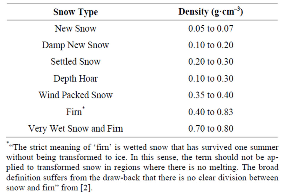
Table 1. Common densities of snow.
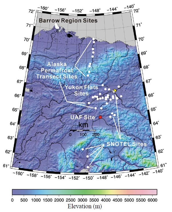
Figure 1. Snow water equivalent measurement sites in Alaska used in this investigation.
2. Satellite-Derived SWE, Model and Ground Measurements in Alaska
2.1. AMSR-E
Spaceborne-derived passive microwave snow water equivalent retrieval is from the Advanced Microwave Scanning Radiometer for the Earth Observation Systems (AMSR-E) developed by the Japan Aerospace Exploration Agency and is[RM6] deployed onboard the NASA Aqua satellite. Daily datasets of global extent are available at the National Snow and Ice Data Center, University of Colorado [5]. We utilize SWE retrievals from version 9 and 10. The datasets comprise grids at 25 km intervals in the EASEGRID projection system [6]. We re-project the grids to the World Geodetic System (WGS) with the WGS-84 ellipsoid.
AMSR-E is a passive microwave scanning radiometer [7]. It operated from NASA Aqua in a polar sun-synchronous (PM, local 13:30 equator crossing time) orbit from June 2002 to 4 October 2011 (Table 2). Microwave frequencies in six channels range from 6.9 to 89 GHz. The instantaneous field of view (IFOV) at the 6.9 GHz channel is 74 by 43 km, and at the 89 GHz channel is 6 by 4 km.
The AMSR-E SWE algorithm is a split-window method using surface brightness temperatures of the 10, 18 and 36 GHz channels in vertical polarization from the Level 2A swath data resampled to 25 km grid [8]. The algorithm first estimates snow depth with adjustment from estimates of forest fraction and density from a global vegetation dataset (Boston University IGBP). Lastly snow density is assumed from a global gridded product derived from hydrologic surveys in Canada (1946-1995) and Russia (1966-1996) and multiplied by the estimate of snow depth. Division by the density of pure water preserves the centimeter unit. Figure 2(a) illustrates AMSRE SWE on 21 March 2011.
2.2. ESA GlobSnow
Beginning in 2008 the European Space Agency Data User Element funded GlobSnow Project strives to assemble a database of Northern Hemisphere snow extent (15 year period) and SWE (30 year period) to aid climate, hydrological and meteorological research [9].
Partner organizations include the Finnish Meteorological Institute, Norwegian Computing Centre, ENVEO IT GmbH, GAMMA Remote Sensing AG, Finnish Environment Institute, Environment Canada and Northern Research Institute.
The GlobSnow SWE is a three-stage model-data assimilation optimization product [10]. The inversion procedure uses the semi-empirical Helsinki University of Technology snow emission model to describe the spaceborne observed microwave brightness temperature of snow cover characteristics (granularity and pore water content) [11]. Data are assimilated from passive micro-
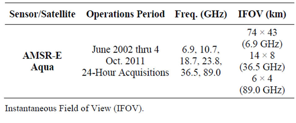
Table 2. Summary characteristics of AMSR-E (NASA aqua [EOS PM]).
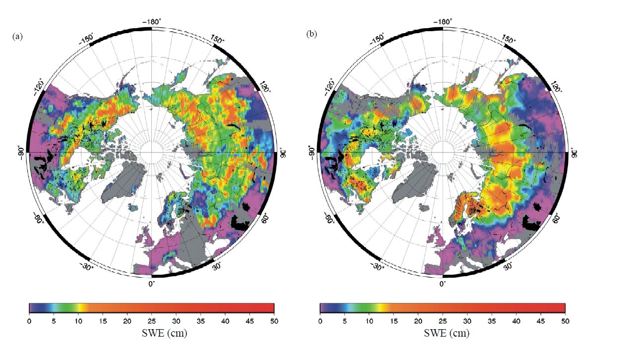
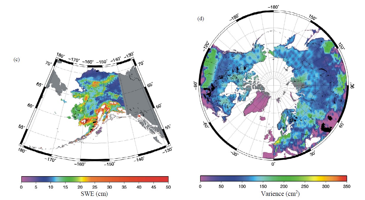
Figure 2. Examples of SWE datasets: (a) AMSR-E on 21 March 2011; (b) GlobSnow on 21 March 2011; (c) GIPL model for March 2011 (mean) and (d) GlobSnow variance on 21 March 2011.
wave-based spaceborne sensors (this case being AMSRE) and ground-based weather station observations of snow depth. The inversion code of the optimization process uses block-averaging and kriging techniques at the weather station location reference measurements [10].
We utilize daily northern hemisphere grids at 25 km intervals in the EASEGRID projection system. For comparison to the other datasets we re-project to the WGS datum. Figure 2(b) illustrates GlobSnow SWE on 21 March 2011. Figure 2(d) illustrates the variance (cm2)
on 21 March 2011. The faint dimple pattern seen in the Alaska and northern Russia sectors indicates the sparse ground network stations used in the kriging processing. The ground network stations are much denser in southern Canada and Russia where the variance is much lower.
2.3. GIPL2-MPI
Geophysical modeling of permafrost has focused on three general methodologies: empirical, equilibrium and numerical [12]. The Geophysical Institute Permafrost Lab (GIPL) permafrost models have evolved into transient numerical methods to incorporate phase changes, moving freezing-thawing boundary and high spatial resolution 2-km grid and temporal resolution at monthly interval [13]. The projection system datum is the WGS- 84 ellipsoid.
SWE, snow density and conductivity are important to permafrost modeling to successfully solve the Stefan heat conduction problem with phase change and moving freeze/thaw boundary [13]. The GIPL2-MPI model code calculates snow density according to [14] with an e-folding time of 4-day. Snow water equivalent is extracted from a 5-GCM composite precipitation dataset covering Alaska [15]. A calibration of model SWE with Alaska ground measurements is performed as a final step. Figure 2(c) illustrates GIPL SWE for March 2011 (mean).
2.4. Barrow Tundra Frozen Lakes
During 21-26 March 2004 snow depth measurements were made on the large tundra frozen lakes east of Barrow [16]. Measurement sites are shown in Figure 3. Snow machines facilitated deployment on days of favorable weather conditions. Global Positioning System Trimble 5700 receivers with survey tri-pods to acquire ele-
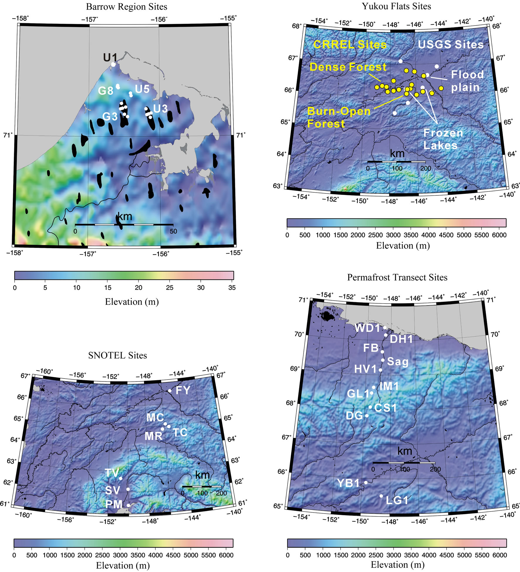
Figure 3. Ground measurement snow water equivalent sites in Alaska.
vation data. Snow depth measurements at 10-m intervals were made along 200 m transects, oriented N-S and E-W with the GPS receivers in the center. We utilize mean snow density of 0.32 g/cm3 measured in March 2003 near Barrow during the AMSR-Ice03 campaign [17].
The Barrow region is a very low relief (~20 m) region of the Alaska Arctic coastal plain. Numerous large NWSE oriented tundra lakes cover the continuous permafrost zone. Vegetation consists of short grasses and mosses.
2.5. University of Alaska Fairbanks Experiment Station
The University of Alaska Fairbanks (UAF) Agriculture and Forestry Experiment Station, formally established by the US Department of Agriculture in 1906, maintains daily meteorological data of surface air temperature, precipitation, extreme events and snow depth [18]. Measurement records from September 1, 1904 are available online through the NOAA National Climate Data Center [19]. The meteorological station is currently located within the experimental agriculture field on the south side of the campus (147.86˚W, 64.85˚N, 150 m elevation, Figure 1 red dot). The terrain surrounding the current met-station the Tanana Flats includes flat lands and modest relief with varied Burch and Spruce stands underlain by discontinuous permafrost with ice-wedge networks.
We utilize daily snow depth during March 2004 through 2009 archived at the UAF Climate Research Center (also at NOAA National Climate Data Center) [20] in keeping with the March 2004 and 2011snow measurement in Alaska. Automated sonic transducer makes the measurements every 24-hour. We assume a mean density of 0.2 g/cm3 to convert snow depth to SWE. Given the relatively large AMSR-E IFOVs in the passive microwave an exact agreement of retrieval-SWE with measured SWE is not expected.
2.6. Yukon Flats Sites
Personnel from the US Army Corps of Engineers Cold Regions Research and Engineering Laboratory (CRREL), US Fish and Wildlife Service and USGS Menlo Park performed snow depth, density and SWE measurements at locations within Yukon Flats (Yukon Flats National Wildlife Refuge) using aircraft transport on 21-25 March 2011 (M. Sturm, C. Hiemstra and M. Waldrop, pers. comm. 2012). This is part of an ongoing multi-disciplinary study under the Yukon River Basin Initiative [21]. Measurement site-locations were selected away from the aircraft in vegetation settings of burn-scar, meadow, open and dense canopy Burch-Spruce forest stands (Figure 3).
The CRREL team performed ten snow depth and density measurements at each location with GPS providing coordinate positioning and noted underlying ground type and surrounding vegetation. The USGS team followed the same procedure for snow depth measurements at their locations. At the USGS locations we assume a mean snow density from the CRREL team.
Yukon Flats is a low relief basin of the Yukon River watershed in eastern Alaska on the Arctic Circle [22]. It is mostly in the discontinuous permafrost zone. Topographically Yukon Flats is bound by the Brooks Range on the north and White Mountains on the south. At the confluence of the Yukon, Porcupine and Chandalar rivers and low relief it is a boreal wetland area, a wildlife refuge with numerous bogs and fens and thermokarst lakes [23].
2.7. Central Alaska SNOTEL Sites
The US Department of Agriculture (USDA) Natural Resources Conservation Service (NRCS) installs, maintains and operates a network of automated SNOwpack TELemetry system in the western Contiguous US and Alaska [24]. We utilize seven of the sixty sites in Alaska, Figure 3. The National Water and Climate Center, USDA coordinates these efforts. SNOTEL had its beginning in 1935 as a snow survey and water supply program within the Soil Conservation Service (predecessor of NRCS). Automated data gathering stations are equipped with snow pillow-pressure transducer for snow water content, sonic sensor for snow depth, precipitation gages and shielded thermistor for near-surface air temperature. Some sites also include sensors for air pressure and relative humidity, solar radiation, near-surface wind fields and soil moisture-temperature. Ground-truth poles allow for periodic validation of snow depth. Data are transmitted in near-real time to regional base stations via VHF radio technology meteor burst communication system. The receiving base station in Alaska is located in Anchorage.
We chose sites from Fort Yukon (FY) to Point Mackenzie (PM), Figure 3. We inspect each site’s data-sensor (snow pillow and sonic sensor) records (hourly) and site characteristics for consistent operation and performance. Errors and degradation of accuracy can occur due to melt of thin snow, high evaporative potential leading to snow-bridging and differential stress on the perimeter during periods of rapid snow settlement or rapid melting [25]. At the Fort Yukon site we adopt a snow density of 0.21 g/cm3 based on our experience in this area. The sites chosen are within the Taiga snow cover class [26]. Vegetation characters include one recently burned area, open and dense forest cover types. Four sites are within the discontinuous permafrost zone and three within the sporadic permafrost zone.
2.8. Alaska Permafrost Transect
During April 2009 and 2010 snow depth and density measurements were taken at locations along the Alaska permafrost transect from Livengood to Prudhoe Bay (Figure 3). At each location nine to twelve measures were performed. Automated meteorological stations and boreholes for measuring ground temperature and active layer thickness occupy the locations.
Since inception in 1977 [27] the Alaska permafrost transect has become part of the US National Science Foundation Arctic Observing Network, the Circumpolar Active Layer Monitoring network, the International Permafrost Association (IPA)—International Polar Year Ther-mal State of Permafrost Project and the IPA Global Terrestrial Network for Permafrost.
3. Results
Comparisons of the ground measured SWE are presented in Figure 4. Plots show comparisons by day-of-month (GIPL is the monthly mean value) and in 1-to-1 comparison (same location). In the plots the symbols are as follows: AMSR-E Blue filled circles, GIPL Yellow filled triangles, Ground Measurements Green filled squares and GlobSnow Open circles.
3.1. Barrow Region
At the measurement sites on the frozen tundra lakes of the Barrow region GlobSnow shows slight over performance relative to ground measurements on average (Figure 4). AMSR-E shows slight under performance relative to ground measurements on average. Winter storm with whiteout conditions occurred on March 23 and 25. Regressions (Table 3) show that both GlobSnow and AMSR-E increase, as do the ground measurements following the days of snowfall events. With no vegetation impeding the retrieval algorithm, AMSR-E has its best performance relative to ground measurements. GIPL model monthly mean SWE shows good agreement with the ground measurements after calibration.
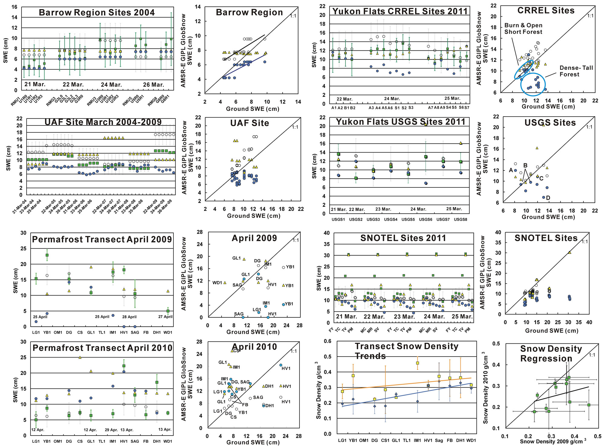
Figure 4. Ground measurement snow water equivalent comparisons to AMSR-E, GlobSnow and GIPL model derived estimates.
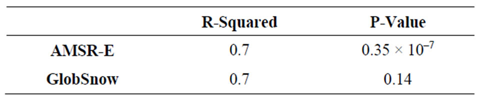
Table 3. Regressions of SWE measurements at barrow tundra frozen lake sites to AMSR-E and GlobSnow SWE estimates.
3.2. UAF Experiment Station
At the UAF experiment station location during March of 2004 through 2009 GlobSnow shows slight over performance relative to measurements through March 2008 and large over performance during March 2009 (Figure 4). Weather conditions of surface wind and near-surface temperature during March 2009 were not exceptional. AMSR-E shows consistent modest underperformance with very small year-to-year variation relative to measurements on average. GIPL model monthly mean SWE shows good agreement to ground measurements through March 2008 with 2009 being an exception (under performance).
3.3. Yukon Flats
At the Yukon Flats locations during March 2011 GlobSnow shows closest agreement to ground measurements with slight over performance, i.e. greater than ground measurements on average (Figure 4, Table 4). AMSR-E shows underperformance, i.e. less than ground measurements on average. In considering the vegetation at the ground locations the AMSR-E underperformance is due from tall dense forest. AMSR-E has its best performance, i.e. closest to ground measurements at location of recent fire burn scars. GIPL model monthly mean SWE falls within the standard deviations of GlobSnow and ground measured SWE.
3.4. Central Alaska SNOTEL Sites
At the Central Alaska SNOTEL locations during March 2011 GlobSnow shows closest agreement to ground measurements with some underperformance, i.e. lessor than ground measurements on average (Figure 4, Table 5). The time series in Figure 4 shows that underperformance grows from Fort Yukon (FY) to Susitna Valley (SV) then lessens at Point Mackenzie (PM). Vegetation conditions and the regional terrain of the foothills of the Alaska Range are likely causes of the underperformance. AMSR-E shows the greatest underperformance on average. AMSR-E underperformance grows from the Fort Yukon site to the Point Mackenzie site and is likely a vegetation-related artifact of the retrieval algorithm. In considering the vegetation at the ground locations AMSR-E and GlobSnow have their best performance, i.e.
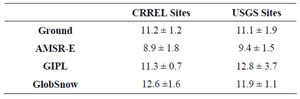
Table 4. Comparisons of SWE mean and standard deviation (cm) yukon flats sites.
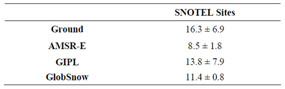
Table 5. Comparisons of SWE mean and standard deviation (cm) at SNOTEL Sites.
closest to ground measurements at the location of the recent fire burn scar at the Monument Creek (MC) site. GIPL model monthly mean SWE was calibrated to ground measured SWE; in this case the plot serves a check of the calibration.
3.5. Alaska Permafrost Transect
At the measurement sites along the transect 65.5˚N to 70.4˚N in complex terrain and vegetation conditions there is no agreement of GlobSnow, AMSR-E or GIPL model to ground measurements in April 2009 and 2010 (Figure 4). This is not unexpected. It has been known for many years that SWE estimated from satellite-based passive microwave sensors has its poorest performance in mountain terrains [28]. The GlobSnow lack of performance is related to the lack of weather stations with snow depth and SWE measurements in mountainous terrain, which are needed for block averaging and kriging.
Plots of the April 2009 and 2010 ground measured snow densities and regressions are given in Figure 4. Inter-site variation of snow density is relatively large. Variation year-to-year is also relative large. There is a significant latitude gradient of snow density from Livengood (65.5˚N) to West Dock (70.4˚N) (Table 6).
4. Discussion
All satellite-based sensor algorithms have simplifying assumptions when retrieving a physical parameter based on surface brightness temperature. A critical factor in the AMSR-E SWE retrieval algorithm is the assumption of snow density from hydrologic snow surveys in Canada (1946-1995) and Russia (1966-1996) [8]. The original data, irregularly spaced, were interpolated to cover the northern hemisphere and sampled on a 25 km interval grid. The Canada survey snow data, network distribution
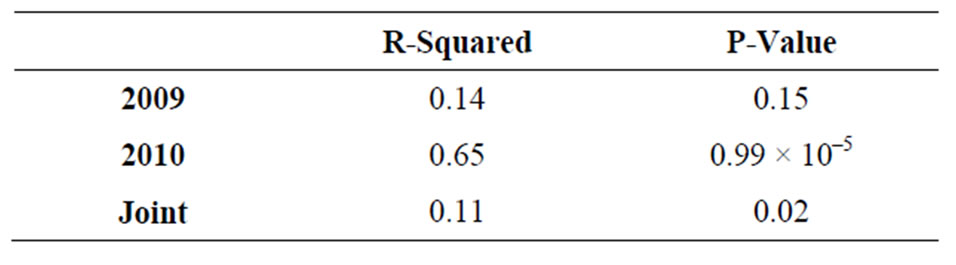
Table 6. Regressions of snow density measurements at Alaska permafrost transect sites.
and spatial properties, have been described in [29]. [30] re-examined them relative to the snow cover classes defined by [26].
Table 7 shows a comparison of mean snow densities per snow cover class and as a percentage difference per snow cover class: April 2009/10 versus Winter 1989- 1991 Alaska [26] and April 1961-1990 Canada [30] and March 2011 versus Winter 1989-1991 Alaska [26] and March 1961-1990 Canada [30]. Large inter-annual decadal differences are noticeable. Regional differences in the Taiga class depending on vegetation cover canopy and stand-density variations are noticeable. Percentage differences show that April 2010 mean density in Taiga class increase 4%, Alpine class decrease 29% and Tundra class increase 33% relative to April 1961-1990. March 2011 mean density in the Taiga class increase up to 15% relative to Winter 1989/90 Alaska and up to 5% relative to March 1961-1990 Canada.
Bulk density of snow depends on compaction, constituents, granularity, humidity, pressure and temperature [1-4,26,31,32]. Snow depth depends on precipitation, surface wind and vegetation [33-35]. Deep snow has the potential for more compaction than thin snow, which can modify bulk snow density.
Our measurements in Alaska show regional variability consistent with temperature variability and elevation at the locations. Interior Alaska typically has colder temperatures in winter relative to the northern Arctic Ocean coast. Relative to the local triple-point of water locations with low temperatures (below the freezing point temperature) correspondingly have low-density snow whereas locations with temperatures closer to the local triplepoint correspondingly have higher density snow. Local temperature and pressure varies with elevation; i.e. alpine fresh snow is less dense relative to valley fresh snow if the other influences are the same. Due to the thermodynamic properties of hexagonal ice and water, snow on the ground during the winter season is changed by metamorphic processes that are in-turn affected by snow pack humidity, surface wind and vegetation cover.
On regional and continental scales and on annual and decadal time intervals seasonal snow cover extent and SWEmax (i.e. maximum SWE) have been shown to be indicators of climate trends [29,30]. In the western sector of North America atmospheric circulation pattern shifts correlate with shifts in the trends of snow cover extent

Table 7. Comparison of mean snow densities (g/cm3) per snow class [26] and percentage change in Alaska and in Canada [30].
and SWEmax.
Our comparisons of snow density per snow cover class show snow density is an indicator of climate and trends. Low elevation Taiga and Tundra snow density is increasing and Alpine snow density is decreasing. This is coupled to precipitation and near-surface temperature trends with variations due to continentality, elevation and vegetation. These factors also affect snow granularity and pore water content, which confer a variation to snow density. Therefore, our measurements and comparisons show that snow density is a non-stationary variable of snow water equivalent.
Inter-satellite and sensor comparisons of SWE retrievals from the Scanning Multichannel Microwave Radiometer, the Special Sensor Microwave/Imager (SSM/I) and AMSR-E shows AMSR-E underperformance across the Arctic [36]. The elevation range in this comparison was from mean-shoreline to 100 m, essentially representing low-elevation tundra with minimal vegetation. If the snow density assumption of the AMSR-E algorithm was not a factor, then there should have been nominal to no SWE underperformance relative to SSM/I on the same locations and times.
5. Conclusions
Our comparisons of satellite-derived, assimilationand model-derived SWE with ground measurements show regional and annual to decadal variations. We show that snow density is an indicator of climate. Snow density responds to trends of temperature, humidity and pressure through the thermodynamic properties of ice (ice Ih) and its varied crystalline forms. Regional trends have spatial variability due to variations of continentality, elevation and vegetation covers. Furthermore, such spatial variations are affected by shifts in atmosphere circulation patterns of the Pacific-North America sector. On annual and decadal intervals snow density is a non-stationary variable of snow water equivalent.
Therefore future satellite-based sensor systems and terrestrial measurement networks should co-develop and evolve together. Using the Global Positioning System as a development model we envision a coordinated-integrated satellite-ground based system for direct measurement of snow density at site-specific, regional and global scales for climate and environment science investigations and geophysical modeling.
6. Acknowledgements
We thank M. Sturm and C. Hiemstra (CRREL), M. Bertram US Fish and Wildlife Service and M. Waldrop (USGS) for contributing the snow datasets of the Yukon Flats National Wildlife Refuge. We thank the US Dept. of Agriculture Natural Resources Conservation Service and National and Water Climate Center for providing the SNOTEL network and data. R. R. Muskett thanks the members of the Geophysical Institute Permafrost Laboratory W. Cable, R. Daanen, E. Jafarov, S. Marchenko and V. Romanovsky for their data contributions to this investigation. R. R. Muskett thanks D. Atwood and C. Lingle 2004 Barrow GPS Campaign funded by a grant from the National Geospatial-Intelligence Agency. V. Romanovsky funded R. R. Muskett by a grant through the USGS Alaska Climate Science Center in coordination with the Arctic and Western Alaska Landscape Conservation Cooperative (A. Maguire and S. Gray USGS) and the Scenarios Network for Alaska and Arctic Planning (S. Rupp UAF). R. R. Muskett thanks the UAF Arctic Region Supercomputing Center for computational facilities assistance. The Generic Mapping Tools were used. Data[RM10] used in the investigation are archived at www.permfrostwatch.org (permafrost.gi.alaska.edu).
REFERENCES
- M. Sturm and C. Benson, “Scales of Spatial Heterogeneity for Perennial and Seasonal Snow Layers,” Annals of Glaciology, Vol. 38, No. 1, 204, pp. 253-260. doi:10.3189/172756404781815112
- W. S. B. Paterson, “The Physics of Glaciers,” 3rd Edition, Butterworth-Heinemann, Boston, 2001.
- V. F. Petrenko and R.W. Whitwort, “The Physics of Ice,” Oxford University Press, New York, 2003.
- H. Bader, “Sorge’s Law of Densification of Snow on High Polar Glaciers,” Journal of Glaciology, Vol. 2, No. 15, 1954, pp. 319-323.
- M. Tedesco, R. E. J. Kelly, J. L. Foster and A. T. C. Chang, “AMSR-E/Aqua Daily L3 Global Snow Water Equivalent EASE-Grids V009 & V010,” National Snow and Ice Data Center, Boulder, 2004.
- http://nsidc.org/data/docs/daac/ae_swe_ease-grids.gd.html
- R. E. Kelly, A. T. Chang, L. Tsang and J. L. Foster, “A Prototype AMSR-E Global Snow Area and Snow Depth Algorithm,” IEEE Transactions on Geoscience and Remote Sensing, Vol. 41, No. 2, 2003, pp. 230-242. doi:10.1109/TGRS.2003.809118
- M. Tedesco and P. S. Narvekar, “Assessment of the NASA AMSR-E SWE Product,” IEEE Journal of Satellite Technology Applicaitons Earth Observation and Remote Sensing, Vol. 3, No. 1, 2010, pp. 141-159. doi:10.1109/JSTARS.2010.2040462
- http://www.globsnow.info/
- J. Pulliainen, “Mapping of Snow Water Equivalent and Snow Depth in Boreal and Sub-Arctic Zones by Assimilating Space-Borne Microwave Radiometer Data and Ground-Based Observations,” Remote Sensing of Environment, Vol. 101, 2006, pp. 257-269. doi:10.1016/j.rse.2006.01.002
- J. Pulliainen, J. Grandell and M. Hallikainen, “HUT Snow Emission Model and Its Applicability to Snow Water Equivalent Retrieval,” IEEE Transactions Geoscience and Remote Sensing, Vol. 37, No. 3, 1999, pp. 1378-1390. doi:10.1109/36.763302
- D. Riseborough, N. Shiklomanov, B. Etzelmuller, S. Gruber and S. Marchenko, “Recent Advances in Permafrost Modeling,” Permafrost and Periglacial Processes, Vol. 19, No. 2, 2008, pp. 137-156. doi:10.1002/ppp.615
- E. E. Jafarov, S. S. Marchenko and V. E. Romanovsky, “Numerical Modeling of Permafrost Dynamics in Alaska Using a High Spatial Resolution Dataset,” The Cryosphere, Vol. 6, No. 3, 2012, pp. 613-624. doi:10.5194/tc-6-613-2012
- D. L. Verseghy, “Class-A Canadian Land Surface Scheme for GCMS, I. Soil Model,” International Journal of Climatology, Vol. 11, No. 2, 1991, pp. 111-133. doi:10.1002/joc.3370110202
- J. E. Walsh, W. L. Chapman, V. Romanovsky, J. H. Christensen and M. Stendel, “Global Climate Model Performance over Alaska and Greenland,” Journal of Climate, Vol. 21, No. 23, 2008, pp. 6156-6174. doi:10.1175/2008JCLI2163.1
- D. K. Atwood, R. M. Guritz, R. R. Muskett, C. S. Lingle, J. M. Sauber and J. T. Freymueller, “DEM Control in Arctic Alaska with ICES at Laser Altimetry,” IEEE Transactions on Geoscience and Remote Sensing, Vol. 45, No. 11, 2007, pp. 3710-3720. doi:10.1109/TGRS.2007.904335
- M. Sturm, J. A. Maslanik, D. K. Perovich, J. C. Stroeve, J. Richter-Menge and T. Markus, “Snow Depth and Ice Thickness Measurements from the Beaufort and Chukchi Seas Collected during the AMSR-Ice03 Campaign,” IEEE Transactions on Geoscience and Remote Sensing, Vol. 44, No. 11, 2006, pp. 3009-3020. doi:10.1109/TGRS.2006.878236
- http://www.uaf.edu/snras/afes/fairbanks-experiment-farm
- http://www.ncdc.noaa.gov/cdo-web/
- http://climate.gi.alaska.edu/index.html
- http://ak.water.usgs.gov/yukon/
- R. G. Stanley, T. S. Ahlbrandt, R. R. Charpentier, T. A. Cook, J. M. Crews, T. R. Klett, P. G. Lillis, R. L. Morin, J. D. Phillips, R. M. Pollastro, E. L. Rowan, R. W. Saltus, C. J. Schenk, M. K. Simpson, A. B. Till and S. M. Troutman, “Oil and Gas Assessment of Yukon Flats, EastCentral Alaska, 2004,” USGS Fact-Sheet No. 2004-3121, USGS, Deptartment of Interior, Washington, 2004.
- http://www.fws.gov/refuges/profiles/index.cfm?id=75635
- National Water and Climate Center, “SNOTEL and Snow Survey Water Supply Forecasting,” US Department of Agriculture, Washington, 2009.
- J. B. Johnson, A. Gelvin and G. L. Schaefer, “An Engineering Design Study of Electronic Snow Water Equivalent Sensor Performance,” Western Snow Conference Proceedings 75th Annual Meeting, Kailua-Kona, 16-19 April 2007, pp. 23-30.
- M. Sturm, J. Holmgren and G. E. Liston, “A Seasonal Snow Cover Classification System for Local and Global Applications,” Journal of Climate, Vol. 8, No. 5, 1995, pp. 1261-1283. doi:10.1175/1520-0442(1995)008<1261:ASSCCS>2.0.CO;2
- T. E. Osterkamp and V. E. Romanovsky, “Evidence for Warming and Thawing of Discontinuous Permafrost in Alaska,” Permafrost And Periglacial Processes, Vol. 10, No. 1, 1999, pp. 17-37. doi:10.1002/(SICI)1099-1530(199901/03)10:1<17::AID-PPP303>3.0.CO;2-4
- J. Dong, J. P. Walker and P. R. Houser, “Factors Affecting Remotely Sensed Snow Water Equivalent Uncertainty,” Remote Sensing of Environment, Vol. 97, No. 1, 2005, pp. 68-82. doi:10.1016/j.rse.2005.04.010
- R. D. Brown and R. O. Braaten, “Spatial and Temporal Variability of Canadian Monthly Snow Depths, 1946- 1995,” Atmosphere-Ocean, Vol. 36, No. 1, 1998, pp. 37- 54. doi:10.1080/07055900.1998.9649605
- R. D. Brown and P. W. Mote, “The Response of Northern Hemisphere Snow Cover to a Changing Climate,” Journal of Climate, Vol. 22, No. 8, 2009, pp. 2124-2145. doi:10.1175/2008JCLI2665.1
- M. Sturm and C. Benson, “Scales of Spatial Heterogeneity for Perennial and Seasonal Snow Layers,” Annals of Glaciology, Vol. 38, No. 1, 2004, pp. 253-260. doi:10.3189/172756404781815112
- T. A. Douglas and M. Sturm, “Arctic Haze, Mercury and the Chemical Composition of Snow across Northwestern Alaska,” Atmosphere Environment, Vol. 38, No. 6, 2004, pp. 805-820. doi:10.1016/j.atmosenv.2003.10.042
- M. Sturm, “Snow Distribution and Heat Flow in Taiga,” Arctic and Alpine Research, Vol. 24, No. 2, 1992, pp. 145-152. doi:10.2307/1551534
- C. Benson and M. Sturm, “Structure and Wind Transport of Seasonal Snow on the Arctic Slope of Alaska,” Annals of Glaciology, Vol. 18, 1993, pp. 261-267.
- J. P. McFadden, G. E. Liston, M. Sturm, R. A. Peilke Sr. and F. S. Chapin III., “Interaction of Shrubs and Snow in Arctic Tundra: Measurement and Models,” Proceedings of a Symposium Held during the Sixth IAHS Scientific Assembly, Maastricht, 18-27 July 2001, pp. 317-325.
- R. R. Muskett, “Multi-Satellite and Sensor Derived Trends and Variation of Snow Water Equivalent on the HighLatitudes of the Northern Hemisphere,” International Journal of Geosciences, Vol. 3, No. 1, 2012, pp. 1-13. doi:10.4236/ijg.2012.31001