Open Journal of Fluid Dynamics
Vol.2 No.4A(2012), Article ID:26353,7 pages DOI:10.4236/ojfd.2012.24A031
Aerodynamic Simulation of Low Mach Turbulent Jets with Lattice Boltzmann Models
School of Energy and Power Engineering, Huazhong University of Science & Technology, Wuhan, China
Email: huofenghuang_11@163.com
Received September 16, 2012; revised October 28, 2012; accepted November 7, 2012
Keywords: Lattice Boltzmann Model; Lagrange Density; Aerodynamic Performance; Guo Model
ABSTRACT
The lattice Boltzmann method (LBM) is a numerical simplification of the Boltzmann equation of the kinetic theory of gases that describes fluid motions by tracking the evolution of the particle velocity distribution function based on linear streaming with nonlinear collision. To verify the reliability and accuracy of the model simulation of incompressible fluid flow, we program to simulate two-dimensional Poiseuille flow which has the analytical solution by using the three mode: D2Q9 model, He-Luo model, Guo model (D2G9). The tests show that the Guo model gives better results. So, in the article, the Guo model is used to stimulate the jet flow field, then the result of which is compared to the result from the experience. The research of this article is the first step to make use of the LBM on the aeroacoutics of jet flow and to provide a theoretical basis on jet aeroacoustics for further study.
1. Introduction
The first two-dimensional discrete lattice gas model was proposed in 1986 by Frisch, Hasslacher and Pomeau (FHP) [1]. The method is numerically stable and inherently parallel, etc., With using it successfully to simulate a few complex physical systems, especially the successful simulation of fluid phenomena, making the method increasingly attention [2]. But the method has statistical noise, does not meet the Galilean invariance and other deficiencies. To overcome these LGA deficiencies, a Lattice Boltzmann method was developed. McNamara and Zanetti (1988) made direct use of the average number of particles or particle distribution functions instead of Boolean variables evolution, which reached a new model, this model is the first lattice Boltzmann model [3], thereby creating a new fluid calculation direction.
Comparing with Navier-Stokes (N-S) equations, Boltzmann equation (BE) has several advantages: First, the BE is applicable even if the medium could not be considered as continuous, such as in simulating rarefied gas flows or multiphase and multicomponent flows. Second, the BE provides clear physical definitions for the equation of state of the fluid, the viscous stress, and the heat conduction from the molecular transport viewpoint. For the N-S equations, these considerations could not be derived directly from the continuum model. In general, the perfect gas equation of state, the Stokes viscous hypothesis, and the Fourier heat conduction relation have to be introduced to solve the equations. Third, there is a large timescale disparity between these two kinds of equations [1].
On the other hand, the macroscopic quantities in the Navier-Stokes equations, such as density, velocity, pressure, and temperature, are affected by the long timescale of the velocity distribution function, which is of the order of about 10−4 s. Consequently, the BE has a much smaller timescale than the Navier-Stokes equations. However, the BE is relatively simple compared to the NavierStokes equations.
In the recent decade, the Lattice-Boltzmann approach has developed quickly, turning into a powerful tool for the simulation of fluid flow [4,5]. Different from the traditional visual top-down method in the calculation of fluid mechanics, the Lattice-Boltzman method uses downtop method with the start from the micro discrete model of fluid. While using the method of Lattice-Boltzman, the fluid is abstracted as a number of micro particles, which may collide and move on the regular discrete lattice in some simple ways.
The key of Constructing LBGK is to choose the right model of equilibrium distribution function. And the key of different LB models is to constructing a corresponding equilibrium distribution function.
Some people propose their model to compute incompressible N-S equation, but their model has their own definition.
DnQb model which is still widely used, was proposed by Qian in 1992 [6]; 1995, Zou and his collaborators proposed a lattice Boltzmann model which could made the calculation of steady incompressible Navier-Stokes equations, it’s called Zou-Hou model [7]; In 1997, Chen and Ohashi promoted the Zuo-Huo model unsteadily and incompressibly to construct a new incompressible Lattice-BoltZman model. We called it Chen-Ohashi mode [8]. They treated the macro speed  in the Zou-Hou definition as a temporary speed, adjusting which the real fluid speed may be figured out by:
 . The basic concept of Chen-Ohashi model is to adjust velocity field with a potential function, which may lead to the correct unsteady and incompressible N-S function. However, a Possion function needs to be figured out in every time step during calculation, which increased the calculated amount of the model.
While Chen-Ohashi model was being suggested, He and Luo suggested another flow Lattice-Boltzmnan model that generally incompressible. Here we call it He-Luo model [9]. The basic concept is to eliminate directly the high-order Mach (caused by the changes of density) in the equilibrium distribution functions. This is an additional limitation out of low Ma number in the He-Luo model. To minimize the influence of artificial compressibility , the additional condition which needs to be satisfied is
 .
.
In 2000, some researchers including Guo Zhaoli construct a Lattice-Boltzmnan model that is able to stimulate general incompressible N-S equations set, which somehow overcome the insufficiency of the above models [4]. Here it’s called Guo model or D2G9 mode.
In the article, the Lattice-Boltzmann and Guo model is used to stimulate the incompressible jet flow field (Ma ≤ 0.3), then the result of which is compared to the result from the experience. The research of this article is the the first step to make use of the LBM on the aeroacoustics of jet flow and to provide a theoretical basis on jet aeroacoustics for further study. The near-field flow physics simulations were performed using self programming, which is based on the LBM kernel. This paper is arranged as follows: Section 2 provides a brief description of the LBM methodology; Section 3 summarizes the grid setup and flow conditions used for LBM and provides results for both the near and far-field flow variables and finally some closing remarks and future work are included in Section 4.
2. Physical Model
Discrete velocity model was established for Lattice Boltzmann method by starting from the concepts and theories of kinetic theory, statistical mechanics, basing on microscopic particle size. It obtained particle distribution function to meet the mass, momentum and energy conservation conditions, then made calculations of the statistical distribution function of particle, it can obtain the pressure, flow rate and other macro variables.
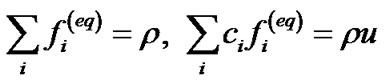
In this paper, as shown in Figure 1, the model of two dimensional nine vectors is discretized into a square. And according to the theory of the Lattice Boltzmann method, it consists of two steps: a streaming step and a collision step.
The time-discrete version of the Boltzmann equation can be written as follows [4]:
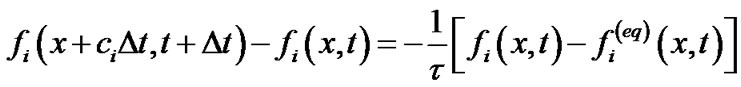 (1)
(1)
Here, in Equation (1), 1 is the particle velocity distribution function,  is dimensionless relaxation time.
  is the equilibrium distribution function of
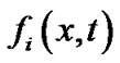 . Equilibrium distribution function of DmQn model has the following general formula:
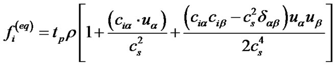 (2)
(2)
Here, in Equation (2),  is constant,
  is weight coefficient.
  is components of the discrete velocity
 . According to Equation (2) shows that, once selected discrete speed
 , equilibrium distribution function can be obtained if one choose the right coefficient
  only. In order to ensure obtaining the correct macro equation, when choosing these weights, it shall be made to meet the mass conservation, momentum conservation and isotropic constraints, so that:
 (3)
(3)
In this model, each node can have three particles stationary particle, orthogonal direction of movement of particles and the diagonal direction of movement of particles,
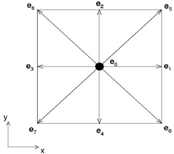
Figure 1. D2Q9 lattice.
respectively. The discrete velocities for the D2Q9 model are defined as . And the nine vectors of the lattice links are documented as follows:
 (4)
(4)
 is Grid speed,
  and
and are the grid step and time step respectively.
The discrete velocity of D2G9 model is still used the discrete velocity of D2Q9 model, but a new class of distribution function was introduced, the equilibrium distribution function was defined as followed [10]:
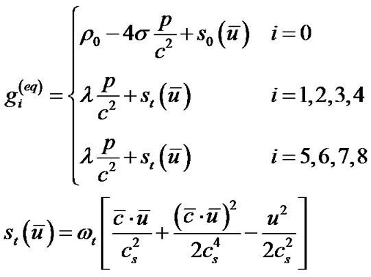 (5)
(5)
 ,
,  ,
,  are some model parameters to meet the conditions:
 (6)
(6)
Throughout the derivation it only meets for low Mach number limit. Meanwhile, comparing with general lattice Boltzmnan model calculation, D2G9’s calculation adds nothing. The model can be applied to unsteady flow.
3. Analysis and Discussion
An overview of the lattice Boltzmann method is provided in the previous section. Based on the above theoretical analysis, we will use D2Q9 model, Guo model (D2G9), He-Luo model to make two-dimensional simulation for constant pressure gradient-driven Poiseuille flow and make comparison with the simulation results and analytical solutions or the existing literature’s data. on the basis of proving Lattice Boltzmann method in proving the calculated value for the fluid stimulation feasibility, several focusing on the comparing basic model simulation results, and from the convergence speed, accuracy, numerical stability analysis of several different angles and compared to choose an excellent model to provide a theoretical basis for further stimulation of jet acoustics by using lattice Boltzmann method.
3.1. Verification Computation
To verify the reliability of the model simulation of incompressible fluid flow, first programming to simulate two-dimensional Poiseuille flow which has the analytical solution.
As show in Figure 2, width is L between the two plates, the fluid viscosity is , flow pressure gradient is
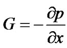 , the analytical solution of flow velocity is:
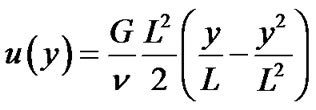 (7)
(7)
Flow region is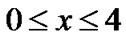 ,
, 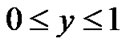 , which is divided by 160 × 40. The fluid initial density
 , initial velocity
 . Pressure boundary conditions for the inlet and outlet [11], the pressure drop gradient
 . After calculation, steady flow can be achieved. By comparing D2Q9 model, He-Luo model, Guo model (D2G9) in use of Poiseuille flow simulation computation, define the analytical solution of Poiseuille flow is
 ,
,  ,
,  ,
,  are respectively D2Q9 model, He-Luo model, Guo model
  simulation results. Define the relative error:
 .
.
As can be seen from the above simulation results (Figure 3), Although D2G9 model though is not too obvious advantage, it is still able to get a more accurate simulation results. Three basic relative errors are not more than 3%, which is within the allowable error range in engineering. From the chart it can also be found that as the Reynolds number increases, D2G9 model errors rise significantly smaller than the other two, the error is much gentler curve, which shows D2G9 model in the large number have significantly higher stability than the rest of the two models at large Re.
3.2. Jet Simulation
The turbulent square jet has been studied experimentally and numerically [12]. The mean streamwise velocity at the center of the slot exit  is 60 (m/s). We will use this data from the experiment in the validation study.
Jet computational domain (excluding the nozzle) grid is designed to: . Grid of Jet compu-
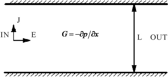
Figure 2. Poiseuille flow schematic diagram.
tational domain is showed in Figure 4. Starting from the prescribed initial conditions, the results are computed for a long enough time to allow for the establishment of statistically stationary turbulent field.
The rate of decrease of the centerline velocity Uax of the jet can be used to make known the extent of penetration [12]. Slow decrease of the centerline velocity would indicate deeper penetration of the jet into the ambiance. Figure 5 showed the computed mean streamwise veloc-
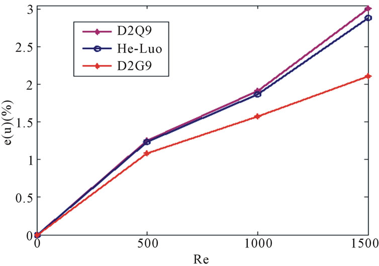
Figure 3. Poiseuille schematic diagram of relative error.
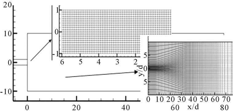
Figure 4. Model and grid computing.
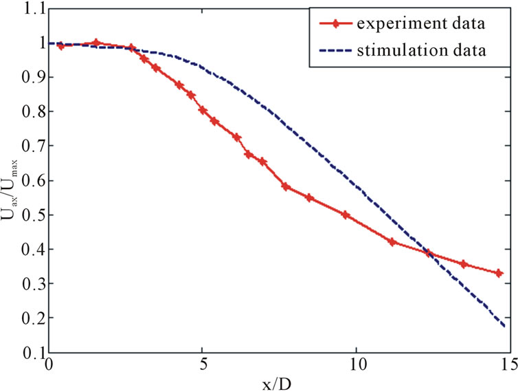
Figure 5. Decay of the mean centerline streamwise velocity Uax (x) normalized by the maximum velocity Umax. The experimental data (blue) are taken from [12].
ity evolution on the jet centerline along with the experimental result of Quinn and Militzer [12]. The centerline velocity Uax is normalized with Umax which is the maximum mean streamwise velocity along the jet center line.
Figure 6 showed the computed variation of the halfwidth with downstream distance along jet centerline. In Figure 6, the velocity half-width  of the jet in the spanwise direction is the distance between the jet centerline and the location where the mean streamwise velocity is half that of the centerline. It is showed that along streamwise direction the trend of between the experimental and LBM results are made very good agreement. The simulations capture the experimental profile reasonably well. Rapid increase of the jet half-width with downstream distance would indicate rapid mixing or spreading. As show in Figure 6, numerical simulation results are smaller than the experimental data.
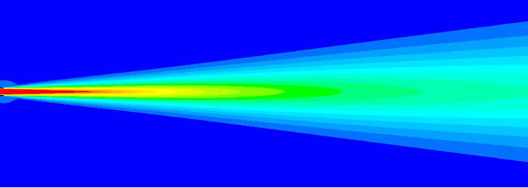
As shown in Figure 7, Visualization process of jet calculation (velocity) shows that the flow goes outside in the xy plane, i.e., along streamwise direction the jet width rapidly extends. In the vertical direction, the flow goes toward the center axis just behind the nozzle, and the jet width is gently extended in the downstream. This feature has also appeared well in the spatially averaged axial velocity profiles (Figure 9).
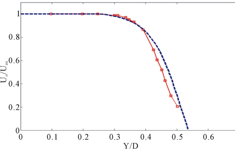
The experimental data (red solid lines) and the numerical results (dashed lines) of Mean streamwise velocity profiles in the central xy plane at different locations are compared in Figure 8. It is noted that all the velocities are dimensionless. Good agreement was obtained with the numerical results for the mean axial velocity.
The spatially averaged axial velocity profiles are displayed in Figure 9. The measured profiles taken at different heights above the outlet follow the free jet theory. Close to the outlet the profile is similar to a turbulent plug flow, with high gradients inside the shear layer. After passing the transition zone for 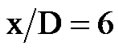 (at the end
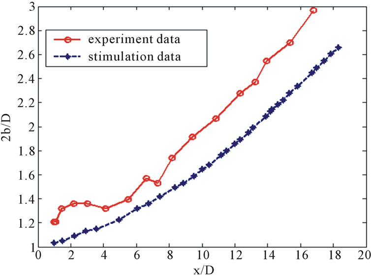
Figure 6. Development of the jet half-width y1/2 along the jet centerline. Experimental (blue) data are taken from [12].
 (a)
(a)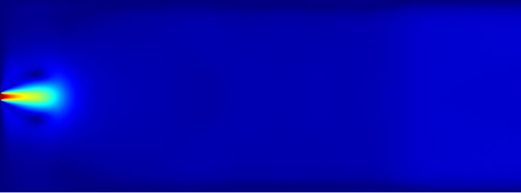 (b)
(b)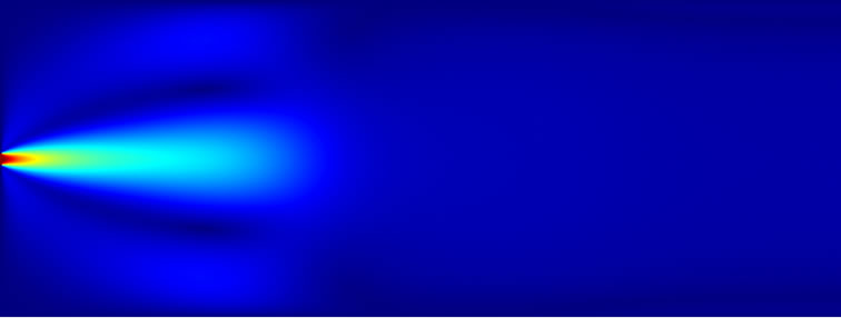 (c)
(c)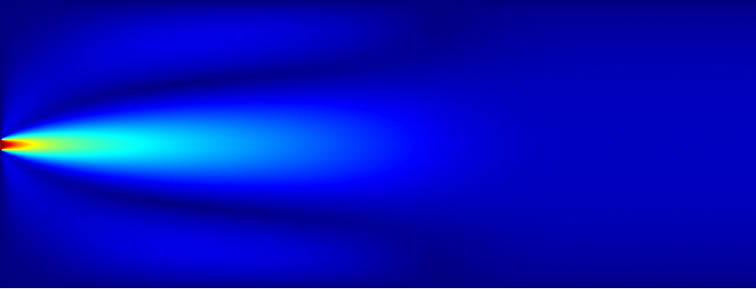 (d)
(d)
Figure 7. Visualization process of jet calculation (velocity).
of the potential core), the jet breaks down with further downstream position, resulting in a typical flattening and broadening of the profile in the starting self-similarity zone .
.
Figure 10 shows comparison of contours of velocity with LES and LBM. It is found that the trend of simulations of LES and LBM is alike. Close to the outlet the profile is similar to a turbulent plug flow, with high gradients inside the shear layer. After passing the transition zone for , the jet breaks down with further downstream position, resulting in a typical flattening and broadening of the profile in the starting self-similarity zone
 . But, compared with traditional CFD, the contours’ line of LBM is smooth transition, and it is equivalent to an ellipse. As the BE provides clear physical definitions for the equation of state of the fluid, the viscous stress, and the heat conduction from the molecular transport viewpoint. So, it is concluded that LBM can better reflect the nature of the fluid flow.
Figures 11 and 12 show the axial turbulence intensities along the centerline and jet shear layer of the jet for both LBM and LES. The simulation results are also compared to recent experimental measurements of Laurendeau et al. [13]. Qualitatively, the trends of the axial turbulence intensities for this jet are consistent with those of an axisymmetric turbulent jet; the peak fluctuation for the centerline occurs earlier and is greater compared to
 (a)
(a)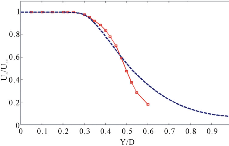 (b)
(b)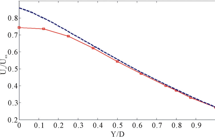 (c)
(c)
Figure 8. Mean streamwise velocity profiles in the central xy plane at different locations. (a) x/D = 0.2; (b) x/D = 2.7; (c) x/D = 4.5. Experimental data (red solid lines) are taken from [12].
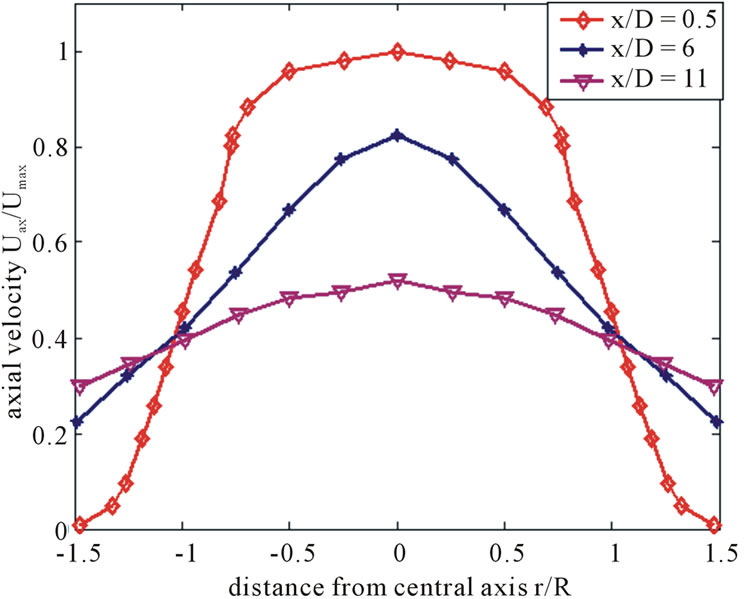
Figure 9. Ensemble averaged filtered axial velocity.
 (a)
(a) (b)
(b)
Figure 10. Comparison of contours of velocity with LES and LBM: (a) LES; (b) LBM.
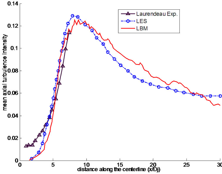
Figure 11. Mean axial turbulence intensity along the jet centerline experiments data are from Laurendeau [13].
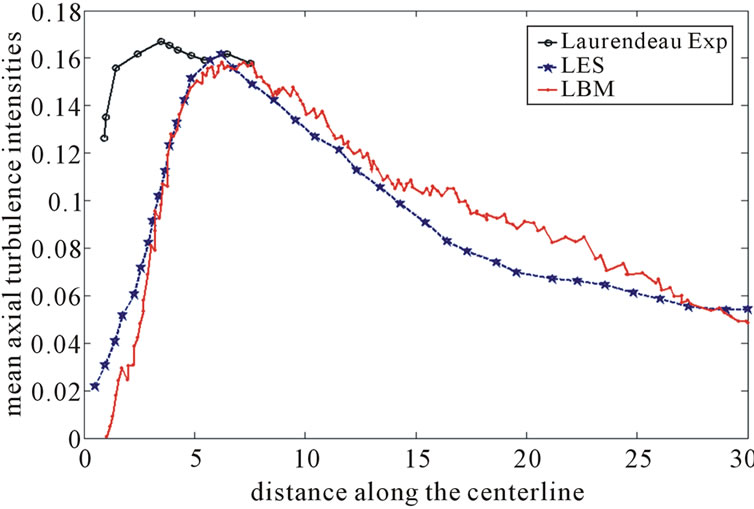
Figure 12. Mean axial turbulence intensity along the jet shear layer for both LBM and LES. Numerical results are compared to the recent experiments of Laurendeau [13].
the centerline peak fluctuation. The decay after the peak intensity is reached is shown to be slightly slower for the LBM compared to the LES. The peak value and the axial location of the computed lip-line turbulence intensity are in agreement with experimental observations.
4. Conclusions
In the article, the LBM is used for numerical simulation of low-Mach jet flow field. Besides, the LBM is used in the first step of research on the aeroacoutics of jet flow, in which the evaluation process of the diffusion and transportation of jet flow is figured out by numerical calculation. This highly reflects the flow in the jet flow filed and the result from the numerical stimulation is coincided with the result of experience.
Of course, practical applications require to run LBM simulations at higher Mach numbers. There is an effort to extend the current lattice-Boltzmann methodology for high Mach number capability. Nonetheless, this study has shown that as a first step towards reaching that goal, the LBM indeed showed promising results for a near compressible jet. Hence, the use of LBM applied to the study of jet aeroacoustics appears to be a viable approach in the field of jet noise simulations.
5. Acknowledgements
T.Y.C. thanks grants from the National Natural Science Foundation of China (No.50976044).
REFERENCES
- U. Frish, B. Hassalacher and Y. Pomeau, “Lattice-Gas Automata for the Navier-Stokes Equation,” Physical Review Letters, Vol. 56, No. 14, 1986, 1505-1508.
- M. Hénon, “Implementation of the FCHC Lattice Gas Model on the Connection Machine,” Journal of Statistical Physics, Vol. 68, No. 3-4, 1992, pp. 353-377. doi:10.1007/BF01341753
- G. R. McNamara and G. Zanetti, “Use of Boltzmann Equation to Simulate Lattice Gas Automata,” Physical Review Letters, Vol. 61, No. 20, 1988, pp. 2332-2335. doi:10.1103/PhysRevLett.61.2332
- Z. L. Guo, B. C. Shi and C. G. Zheng, “A Coupled LBGK Model for the Boussinesq Equations,” International Journal for Numerical Methods in Fluids, Vol. 39, No. 4, 2002, pp. 325-342. doi:10.1002/fld.337
- M. A. Moussaoui, M. Jami, A. Mezrhab and H. Naji, “MRT-Lattice Boltzmann Simulation of Forced Convection in a Plane Channel with an Inclined Square Cylinder,” International Journal of Thermal Sciences, Vol. 49, No. 1, 2010, pp. 131-142. doi:10.1016/j.ijthermalsci.2009.06.009
- Y. H. Qian, D. D’Humières and P. Lallemand, “Lattice BGK Models for Navier-Stokes Equation,” Europhysics Letters, Vol. 17, No. 6, 1992, pp. 479-484. doi:10.1209/0295-5075/17/6/001
- Q. Zou, S. Hou, S. Chen and G. D. Doolen, “An Improved Incompressible Lattice Boltzmann Model for Time-Independent Flow,” Journal of Statistical Physics, Vol. 81, No. 1-2, 1995, pp. 35-48. doi:10.1007/BF02179966
- Y. Chen and H. Ohashi, “Lattice-BGK Methods for Simulating Incompressible Fluid Flows,” International Journal of Modern Physics C, Vol. 8, No. 4, 1997, pp. 793-803. doi:10.1142/S0129183197000680
- X. Y. He and L.-S. Luo, “Lattice Boltzmann Model for the Incompressible Navier-Stokes Equation,” Journal of Statistical Physics, Vol. 88, No. 3, 1997, pp. 927-944. doi:10.1023/B:JOSS.0000015179. 12689.e4
- Z. L. Guo, B. C. Shi and N. C. Wang, “Lattice BGK Model for Incompressible Navier-Stokes Equation,” Journal of Computational Physics, Vol. 165, No. 1, 2000, pp. 288-306. doi:10.1006/jcph.2000.6616
- Q. S. Zou and X. Y. He, “On Pressure and Velocity Boundary Conditions for the Lattice Boltzmann BGK Model,” Physics of Fluids, Vol. 9, No. 6, 1997, pp. 1591- 1598.
- W. R. Quinn and J. Militzer, “Experimental and Numerical Study of a Turbulent Free Square Jet,” Physics of Fluids, Vol. 31, No. 5, 1988, pp. 1017-1025. doi:10.1063/1.867007
- E. Laurendeau, J. P. Bonnet, P. Jordan and J. Delville, “Impact of Fluidic Chevrons on the Turbulence Structure of a Subsonic Jet,” 3rd AIAA Flow Control Conference, San Francisco, 5-8 June 2006, 13 pp.