Journal of Computer and Communications
Vol.04 No.04(2016), Article ID:65949,14 pages
10.4236/jcc.2016.44013
Chronically Evaluated Highest Instantaneous Priority Next: A Novel Algorithm for Processor Scheduling
Amit Pandey, Pawan Singh, Nirayo H. Gebreegziabher, Abdella Kemal
School of Informatics, IOT, Hawassa University, Hawassa, Ethiopia

Copyright © 2016 by authors and Scientific Research Publishing Inc.
This work is licensed under the Creative Commons Attribution International License (CC BY).
http://creativecommons.org/licenses/by/4.0/


Received 13 March 2016; accepted 24 April 2016; published 27 April 2016
ABSTRACT
This paper proposes a novel chronically evaluated highest instantaneous priority next processor scheduling algorithm. The currently existing algorithms like first come first serve, shortest job first, round-robin, shortest remaining time first, highest response ratio next and varying response ratio priority algorithm have some problems associated with them. Some of them can lead to endless waiting or starvation and some of them like round-robin has problem of too many context switches and high waiting time associated with them. In the proposed algorithm, we have taken care of all such problems. As the novel algorithm is capable of achieving as good results as shortest remaining time first algorithm and also it will never lead to starvation.
Keywords:
Chronically Evaluated Highest Instantaneous Priority Next, CEHIPN, Priority Scheduling, Preemptive Scheduling, Processor Scheduling, Starvation

1. Introduction
Scheduling algorithm improves processor’s efficiency by improving its utilization. The short-term scheduler uses various algorithms to do assignments for the processor [1] . First come, first serve (FCFS) [2] - [4] , Shortest job first (SJF) [2] - [5] , Shortest remaining time first (SRTF) [3] [4] , Round-robin (RR) [2] - [4] , Highest response ratio next (HRRN) [4] , Mid Average Round-Robin (MARR) [6] , Adaptive Round-Robin (Adaptive RR) [7] , Improved Round-Robin Approach using Dynamic Time Quantum (IRRADTQ) [8] and Varying Response Ratio Priority (VRRP) [9] , are some of the examples of scheduling algorithm used by the scheduler. A good scheduling approach fulfills some basic goals like increasing throughput, reducing overhead, avoiding starvation and execution according to priority. That is why researchers are working around the world to improve them in the terms of better waiting time and response time.
As performance of the algorithm may vary under various situations [5] , so the possible criteria for selection of a proper algorithm can be reduced context switch count, increased throughput, increased processor use, reduced waiting time, reduced response time and reduced turnaround time [10] .
On analyzing the existing algorithms we found that they have some withdrawing factors, such as long waiting time or starvation associated with them. To overcome these demerits, we have proposed a novel algorithm for processor scheduling. The novel algorithm considers the instantaneous waiting time and instantaneous remaining time for evaluating the priority. The proposed approach is preemptive and the priority for the processes will be calculated when any new process arrives or any process finishes.
2. Related Work
The First come first serve is one of the simplest processor scheduling algorithms [3] [4] , it takes processes in same sequence as they arrive, regardless of their burst time, later it follows the same sequence to assign processor to them. There is a major drawback associated as it is a non preemptive approach less time-consuming process waits for a less important one to finish first.
To overcome this problem the shortest job first algorithm was proposed in which the job with shorter burst time is executed first [3] [4] [11] . But in this approach if short processes keep coming in sequence, then any long process has to wait endlessly for its chance and may starve [12] . Further, there was a new algorithm proposed by the name Shortest remaining time first [3] [4] this was a preemptive approach in which job with shorter remaining time is executed first. Again problem was the same, if new jobs with shorter running time keep coming then an older job with larger remaining time has to wait endlessly creating a condition of starvation.
To overcome this starvation problem new Round-robin algorithm was introduced [3] [4] [11] . In this approach processor handles each process in recurring order and for a fixed time quantum. Hence each process gets the processor equally and no process ever starves. But because of these frequent switching this algorithm is associated with a large number of context switches and high average waiting time [4] [13] . To further reduce the average waiting time, many improvements over round-robin algorithm were proposed [14] - [16] . Like Proportional Share Scheduling Algorithm, which was proposed by Helmy and Dekdouk [16] , this algorithm inherits features from round-robin and is encouraging for shorter jobs, there is an SBRRR algorithm that is a blend of Shortest job first and Round-robin [18] , on the other hand the PBDRR algorithm holds the features from priority algorithm and Round-Robin [19] .
In adaptive Round-Robin [7] [20] , the processes in ready queue are first arranged in increasing order of their burst time. If number of contributing processes is even. Then time quantum is calculated as an average of their burst time. If the number of processes is odd, then burst time of the middle process is taken as the time quantum. Later in mid average Round-Robin algorithm [6] [20] first all processes are sorted in increasing order of their burst time in the ready queue. Next we find the middle process. Then average burst time for all process from mid process to the end process is calculated. This average value is then assigned as a time quantum for further calculations. Further, in 2013, Negi et al. proposed an enhanced Round-Robin algorithm using dynamic time quantum and improved average waiting time [8] . This approach uses a time margin to check whether the process in its second last round can be finished in the same round by extending the time quantum by a small margin. If it is possible then it will be finished in the same round by providing time extension for achieving better performance.
Next in the sequence is the highest response ratio next algorithm [4] . It is a non preemptive approach which considers the ratio of waiting time to burst time for calculating response ratio. This ratio is used to assign next process to the processor. Waiting time is considered for calculating the response ratio. Ensuring process with larger waiting time will get a higher response ratio and it will never starve.
In 2015, Singh et al. Proposed Varying Response Ratio Priority algorithm. It calculates the priority of each process based on their waiting time and remaining burst time [9] . The algorithm ensures there will be no endless waiting by including waiting time in calculating the priority.
The novel algorithm proposed in this paper inherits some features from both highest response ratio next as well as shortest remaining time first approaches. The proposed approach is a preemptive approach. It uses instantaneous remaining time and waiting time together to calculate instantaneous priority.
3. Proposed Approach
The proposed chronically evaluated highest instantaneous priority next algorithm is a preemptive approach. It takes the instantaneous remaining time and waiting time of the processes into consideration to calculate their instantaneous priority. Then the process with highest instantaneous priority is allocated to the processor. This also makes this approach a priority base scheduling algorithm.
The Algorithm
The flow chart included below explains the working of the proposed algorithm (see Figure 1). It can be observed in the flow chart below that each time any process finishes or any new process arrives the instantaneous priority for each participating process will be calculated and then the processor will allocated to the process which has the highest priority.

Figure 1. Flow chartexplaining the CEHIPN algorithm.
4. Functioning of the Algorithm
The proposed algorithm considers two factors instantaneous remaining time and waiting time to calculate the instantaneous priority. Every time either a process finishes or a new one arrives, the priority for every contributing process is calculated.
 (1)
(1)
where,
 = Instantaneous waiting time of the processes.
BT = Burst Time
 = Instantaneous remaining time of processes.

Here, P represents the process number for “n” contributing processes and Rem.T is their respective remaining time. First the sum of remaining time from process 1 to n is calculated. Then the sum is divided by “n” to get mean value as Mean Rem.T. When waiting time of any process increases its priority will also increase. As no process has to wait endlessly. Hence,
 α
α
Time will come when chronically increasing priority of that process will become considerably high to take over the processor from any other process with even smaller remaining time. This is called inversion of execution order.
The priority value will also increase with decreasing remaining time of any process, as shorter jobs should be executed first. Hence,
 α
α
The exponent “n” in the denominator of the formula for calculating instantaneous priority is there to lowers the sharp growth of priority value for any process which has large waiting time. For the higher value of “n” the whole denominator term will become a huge value. Hence even for the process with large waiting time the priority will not increase sharply. This will make the priority value to increase slowly and the priority inversion will be delayed. Which will eventually enhance the performance by keeping the average waiting time for the process low. In the formula the constant 1 is added to the first ratio, so that when the waiting time of any process is zero the value of the first factor will become one. As initially when processes will arrive their waiting time
will be zero. Hence the factor  will become one and the priority for the processes will be simply calculated on the basis of the ratio
 . That is the process with the smallest remaining time will get the highest priority. Also the factor
  is included in formula to scale the priorities.
By scaling we mean to arrange all the processes on same scale with respect to the mean remaining time value. This will help to measure the processes priority on the same scale for getting a proper response. So the second ratio arranges the processes in order to which the enhancement values obtained from the first ratio are multiplied to obtain the instantaneous priority.
Let there be “I” number of processes initially in ready queue as . Let Pk be the process with highest burst time of Tk and sum of burst time for all (i-1) processes except Pk is
 . Then for best performance of CEHIPN we will consider the below equation based on the first factor (See expression 2),

Or,
 (2)
(2)
Now this expression 2 will be used to decide the value of exponent “n” in the formula.
During the run, cases may arise when processes may have same priority. In such cases process with shorter remaining time should be preferred, as it will make CEHIPN to behave like shortest remaining time first algorithm. If their remaining time is also same then any of the process can be chosen. Hence in this case of equality of process priority the below equality holds,
 (3)
(3)
On rearranging the above expression, we will have,
 (4)
(4)
4.1. CASE I: Process Priorities Are Equal and Also Rem.Ti = Rem.Tj
When remaining time of the processes is same, then in expression 4 mentioned above we have,

Let,

Now the expression 4 can be rewritten as,
 (5)
(5)
Or, 
Or,
 (6)
(6)
Therefore, when remaining time is same for both the processes then their waiting time will also be same. Hence anyone of them can be considered for next execution.
4.2. CASE II: Process Priorities are Equal and Also Rem.Ti > Rem.Tj
In this case, when both processes are having different remaining time but same priority. We can recall expression 4,

Now, 
As given that, 
Hence,
 (7)
(7)
Or,
 (8)
(8)
Expression 8 shows that waiting time of Pi is also greater than that of Pj. But priority of both the processes is still same. In this case, the process with smaller remaining time value will be selected next, as waiting time is included in expression 1 to increase the priority to avoid starvation only.
Consider the average waiting time at current instance as AWT for 'm' number of contributing processes. Now if process Pi with larger remaining time is executed first instead of Pj. Then average waiting time at the end, when both processes will finish, will be AWT(i). where,

On the other hand if Pj is executed first. Then average waiting time at the end, when both processes will finish, will be AWT(j). where,

Since Rem.Ti is greater than Rem.Tj. Hence AWT(i) will also be greater than AWT(j). We also know that average waiting time should be kept to minimum for the best performance. Hence second approach of selecting Pj will give better result. Therefore, when priority is same and it comes to selection between two processes. Then process with shorter remaining time will be selected first.
5. Performance of the Algorithm
The performance of the algorithm can be analyzed by comparing the average waiting time, average response time and number of context switches of CEHIPN with other algorithms. We have considered the burst time of the processes in increasing, decreasing and random orders to generate four different cases. Then theoretical calculations are performed to obtain below data for analysis.
5.1. CASE I: Random Order of Burst Time
In Case I processes are arriving in random order of burst time and exponent “n” will take three different values 1, 2 and 3 respectively for three different calculations (see Table 1 and Table 2). It is possible with CEHIPN algorithm to achieve the same results as shortest remaining time first algorithm by varying the values of exponent “n” (see Figure 2 and Figure 3).

Table 1. Random order of burst time―Case I.
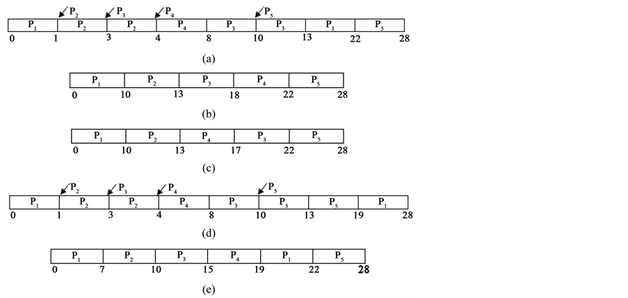
Figure 2. Gantt charts when Burst Time is in Random Order for Case I-Part I. (a) Gantt chart for CEHIPN with Random Order of Burst Time; (b) Gantt chart for FCFS with Random Order of Burst Time; (c) Gantt chart for SJF with Random Order of Burst Time; (d) Gantt chart for SRTF and CEHIPN n = 2, 3 with Random Order of Burst Time; (e) Gantt chart for RR with Random Order of Burst Time.

Figure 3. Gantt charts when burst time is in random order for Case I-Part II. (a) Gantt chart for HRRN with Random Order of Burst Time; (b) Gantt chart for VRRP with Random Order of Burst Time; (c) Gantt chart for MARR with Random Order of Burst Time; (d) Gantt chart for Adaptive RR with Random Order of Burst Time.
Table 2. Data for random order of burst time―Case I.
Calculations Involved in CEHIPN for n = 1:
Round #1: Time = 1 (P2 arrives)
Priority P1 = 0.67
Priority P2 = 2
P2 is selected.
Round #2: Time = 3 (P3 arrives)
Priority P1 = 0.68
Priority P2 = 5
Priority P3 = 1
P2 is selected.
Round #3: Time = 4 (P2 finished and P4 arrives)
Priority P1 = 0.89
Priority P3 = 1.44
Priority P4 = 1.5
P4 is selected.
Round #4: Time = 8 (P4 finished)
Priority P1 = 1.38
Priority P3 = 2.8
P3 is selected.
Round #5: Time = 10 (P5 arrives)
Priority P1 = 1.33
Priority P3 = 5.33
Priority P5 = 1
P3 is selected.
Round #6: Time = 13 (P3 finished)
Priority P1 = 1.94
Priority P5 = 1.88
P1 is selected. Here the priority of P1 got amplified, as it was waiting for a long time. It got selected over P5 which even has a smaller remaining time. Ensuring there will be no starvation.
5.2. CASE II: Random Order of Burst Time
Also in Case II the processes are arriving in random order of burst time and value of exponent “n” in three different calculations of CEHIPN is 1,2 and 3 respectively (see Table 3 and Table 4). On increasing the value of exponent “n”. The result of CEHIPN will improve and will become same as for Shortest remaining time first (see Figure 4 and Figure 5).
5.3. CASE III: Decreasing Order of Burst Time
In Case III the processes are arriving in decreasing order of burst time (see Table 5 and Table 6). The exponent “n” has two values 1 and 3 respectively for two different calculations (see Figure 6 and Figure 7).
Table 3. Random order of burst time―Case II.

Figure 4. Gantt charts when burst time is in random order for Case II- art I. (a) Gantt chart for CEHIPN with random order of burst time and n = 1; (b) Gantt chart for CEHIPN with random order of burst time and n = 2; (c) Gantt chart for FCFS with random order of burst time; (d) Gantt chart for SJF with random order of burst time; (e) Gantt chart for SRTF and CEHIPN n=3 with random order of burst time.

Figure 5. Gantt charts when burst time is in random order for Case II-Part II. (a) Gantt chart for RR with random order of burst time; (b) Gantt chart for HRRN with Random Order of Burst Time; (c) Gantt chart for VRRP with random order of burst time; (d) Gantt chart for MARR with random order of burst time; (e) Gantt chart for adaptive RR with random order of burst time.
5.4. CASE IV: Increasing Order of Burst Time
In this case we will get same values for all the algorithms. As the burst time is in increasing order. So the shorter job will always come first and will be executed first, resulting in same sequence as for the shortest remaining time first algorithm (see Table 7 and Table 8).

Figure 6. Gantt charts for decreasing order of burst time-Part I. (a) Gantt chart for CEHIPN with decreasing order of burst time; (b) Gantt chart for FCFS with decreasing order of burst time; (c) Gantt chart for SJF with decreasing order of burst time; (d) Gantt chart for SRTF and CEHIPN n = 3 with decreasing order of burst time; (e) Gantt chart for RR with decreasing order of burst time.
Table 4. Data for random order of burst time―Case II.
Table 5. Decreasing order of burst time.

Figure 7. Gantt charts for decreasing order of burst time-Part II. (a) Gantt chart for HRRN with decreasing order of burst time; (b) Gantt chart for VRRN with decreasing order of burst time; (c) Gantt chart for MARR with decreasing order of burst time; (d) Gantt chart for adaptive RR with decreasing order of burst time.
Table 6. Data for decreasing order of burst time.
Table 7. Increasing order of burst time.
Table 8. Data for increasing order of burst time.
6. Results
In the present study there is comparison of the novel CEHIPN algorithm with First come first serve, Shortest job first, Shortest remaining time first, Round-robin, Highest response ratio next, Varying Response Ratio Priority, Mid Average Round-Robin and Adaptive Round-Robin in terms of number of context switches, average waiting time, and average response time. There are four different cases where the Burst time of the contributing processes is arranged in random, decreasing and increasing orders to get the following results.
In Figure 8 there is comparison of CEHIPN when processes are arriving in random order of their burst time for Case I (see Figure 8). The average waiting time and average response time of CEHIPN with n = 1 are far better than that of First come first serve, Shortest job first, Round-robin, Highest response ratio next, Varying Response Ratio Priority, Mid Average Round-Robin and Adaptive Round-Robin. For CEHIPN with n = 2 and 3, values are same to that of Shortest remaining time first. The context switches in all the three cases of CEHIPN are less than that of Varying Response Ratio Priority and are equal to that of Shortest remaining time first.
In Figure 9 there is comparison of CEHIPN when processes are arriving in random order of their burst time for Case II and n = 1, 2 and 3 respectively for three cases of CEHIPN (see Figure 9). The average waiting time and average response time of CEHIPN with n = 2 are better than that of CEHIPN with n = 1, First come first serve, Shortest job first, Round-robin, Highest response ratio next, Varying Response Ratio Priority, Mid Average Round-Robin and Adaptive Round-Robin. For CEHIPN with n = 3, values are same to that of Shortest remaining time first. The number of context switches for all three cases of CEHIPN is same as that of Shortest remaining time first and Varying Response Ratio Priority.
In Figure 10 there is comparison of CEHIPN when the burst time is in decreasing order (see Figure 10). The average waiting time of CEHIPN for n = 1 is better than that of First come first serve, Round-robin, Highest response ratio next, Varying Response Ratio Priority, Mid Average Round-Robin and Adaptive Round-Robin. When comparing the average response time the value of CEHIPN with n = 1 is better than First come first serve, Shortest job first, Round-robin, Highest response ratio next, Varying Response Ratio Priority, Mid Average Round-Robin and Adaptive Round-Robin. For CEHIPN with n = 3, values are same to that of Shortest remaining time first. The number of context switches in both the cases of CEHIPN is same as that of Shortest remaining time first and Varying Response Ratio Priority.
In case IV when processes are arranged in increasing order of their burst time, the average waiting time, average response time and the number of context switches for all the considered algorithms are same.
7. Conclusions
From the results of our study it is inferred that CEHIPN has much better results in terms of average waiting time, and average response time, when compared with First come first serve, Shortest job first, Round-robin, Highest response ratio next, Varying Response Ratio Priority, Mid Average Round-Robin and Adaptive Round-Robin. Also for higher values of exponent “n”, CEHIPN gives same results as Shortest remaining time first, until there

Figure 8. Comparison for Case I : Burst time in random order.

Figure 9. Comparison for Case II : Burst time in random order.

Figure 10. Comparison when burst time is in decreasing order.
is no inversion of execution order. On the other hand, the number of context switches associated with CEHIPN is same as for Shortest remaining time first. Also the proposed CEHIPN algorithm will never lead to starvation.
In the present study it is concluded that novel CEHIPN algorithm is better than First come first serve, Shortest job first, Round-robin, Highest response ratio next, Varying Response Ratio Priority, Mid Average Round- Robin and Adaptive Round-Robin in terms of average waiting time and average response time. For higher values of exponent “n” CEHIPN gives result same as Shortest remaining time first, until there is no inversion of execution order and also it will never lead to starvation.
Cite this paper
Amit Pandey,Pawan Singh,Nirayo H. Gebreegziabher,Abdella Kemal, (2016) Chronically Evaluated Highest Instantaneous Priority Next: A Novel Algorithm for Processor Scheduling. Journal of Computer and Communications,04,146-159. doi: 10.4236/jcc.2016.44013
References
- 1. Stallings, W. (2009) Operating Systems (Vol. 6). Pearson Education, New York, 72-73.
- 2. Nutt, G. (2003) Operating Systems (Vol. 3). Pearson, New York, 204-212.
- 3. Silberschatz, A., Galvin, P.B. and Gagne, G. (2001) Operating System Concepts (Vol. 6). Wiley, Hoboken, 151-184.
- 4. Deitel, H.M. (1984) An Introduction to Operating Systems (Vol. 1). Addison-Wesley, Reading, MA, 248-259.
- 5. Oyetunji, E.O. and Oluleye, A.E. (2009) Performance Assessment of Some CPU Scheduling Algorithms. Research Journal of Information and Technology, 1, 22-26.
- 6. Banerjee, P., Banerjee, P. and Dhal, S.S. (2012) Comparative Performance Analysis of Mid Average Round Robin Scheduling (MARR) Using Dynamic Time Quantum with Round Robin Scheduling Algorithm Having Static Time Quatum. International Journal of Electronics and Computer Science Engineering, 1, 2026-2034.
- 7. Hiranwal, S. and Roy, K.C. (2011) Adaptive Round Robin Scheduling Using Shortest Burst Approach, Based on Smart Time Slice. International Journal of Computer Science and Communication, 2, 319-323.
- 8. Negi, S. (2013) An Improved Round Robin Approach Using Dynamic Time Quantum for Improving Average Waiting Time. International Journal of Computer Applications, 69, 12-16.
http://dx.doi.org/10.5120/11909-8007 - 9. Singh, P., Pandey, A. and Mekonnen, A. (2015) Varying Response Ratio Priority: A Preemptive CPU Scheduling Algorithm (VRRP). Journal of Computer and Communications, 3, 40.
http://dx.doi.org/10.4236/jcc.2015.34005 - 10. Rajput, I.S. and Gupta, D. (2012) A Priority Based Round Robin CPU Scheduling Algorithm for Real Time Systems. International Journal of Innovations in Engineering and Technology, 1, 1-11.
- 11. Tanenbaum, A.S. and Woodhull, A.S. (1996) Operating Systems Design and Implementation (Vol. 2). Pearson, New York, 82-88.
- 12. Shahzad, B. and Afzal, M.T. (2006) Optimized Solution to Shortest Job First by Eliminating the Starvation. In Proceedings of the 6th Jordanian Inr. Electrical and Electronics Eng. Conference (JIEEEC 2006), Jordan.
http://www.researchgate.net/publication/234556241_OPTIMIZED_SOLUTION_TO_SHORTEST_JOB_FIRST_BY_ELIMINATING_THESTARVATION - 13. Yadav, R.K., Mishra, A.K., Prakash, N. and Sharma, H. (2010) An Improved Round Robin Scheduling Algorithm for CPU Scheduling. International Journal on Computer Science and Engineering, 2, 1064-1066.
- 14. Singh, A., Goyal, P. and Batra, S. (2010) An Optimized Round Robin Scheduling Algorithm for CPU Scheduling. International Journal on Computer Science and Engineering, 2, 2383-2385.
- 15. Noon, A., Kalakech, A. and Kadry, S. (2011) A New Round Robin Based Scheduling Algorithm for Operating Systems: Dynamic Quantum Using the Mean Average. International Journal of Computer Science Issues, 8, 224-229.
- 16. Behera, H.S., Swain, B.K., Parida, A.K. and Sahu, G. (2012) A New Proposed Round Robin with Highest Response Ratio Next (RRHRRN) Scheduling Algorithm for Soft Real Time Systems. International Journal of Engineering and Advanced Technology, 37, 200-206.
- 17. Helmy, T. and Dekdouk, A. (2007) Burst Round Robin as a Proportional-Share Scheduling Algorithm. Proceedings of the 4th IEEE-GCC Conference on Towards Techno-Industrial Innovations, Bahrain, November 2007, 424-428.
- 18. Mohanty, R., Behera, H.S., Patwari, K. and Dash, M. (2010) Design and Performance Evaluation of a New Proposed Shortest Remaining Burst Round Robin (SRBRR) Scheduling Algorithm. Proceedings of International Symposium on Computer Engineering & Technology (ISCET), 17, 126-137.
www.rimtengg.com/iscet/proceedings/pdfs/advcomp/126.pdf - 19. Mohanty, R., Behera, H.S., Patwari, K., Dash, M. and Prasanna, M.L. (2011) Priority Based Dynamic Round Robin (PBDRR) Algorithm with Intelligent Time Slice for Soft Real Time Systems. International Journal of Advanced Computer Science and Applications, 2, 46-50.
http://dx.doi.org/10.14569/IJACSA.2011.020209 - 20. Negi, S. and Kalra, P. (2014) A Comparative Performance Analysis of Various Variants of Round Robin Scheduling Algorithm. International Journal of Information & Computation Technology, 4, 765-772.