Received 9 November 2015; accepted 24 January 2016; published 27 January 2016

ABSTRACT

A standard assumption in the literature of learning theory is the samples which are drawn independently from an identical distribution with a uniform bounded output. This excludes the common case with Gaussian distribution. In this paper we extend these assumptions to a general case. To be precise, samples are drawn from a sequence of unbounded and non-identical probability distributions. By drift error analysis and Bennett inequality for the unbounded random variables, we derive a satisfactory learning rate for the ERM algorithm.

Keywords:

Learning Theory, ERM, Non-Identical, Unbounded Sampling, Covering Number

1. Introduction

In learning theory we study the problem of looking for a function or its approximation which reflects the relationship between the input and the output via samples. It can be considered as a mathematical analysis of artificial intelligence or machine learning. Since the exact distributions of the samples are usually unknown, we can only construct algorithms based on an empirical sample set. A typical setting of learning theory in mathe- matics can be like this: the input space X is a compact metric space, and the output space for regression. (When,it can be regarded as a binary classification problem.) Then is the whole sample space. We assume a distribution on Z, which can be decomposed to two parts: marginal distribution on X and conditional distribution given some. This implies

for any integrable function [1] .

To evaluate the efficiency of a function we can choose the generalization error:

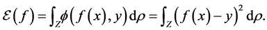
Here is a loss function which measures the difference between the prediction via f and the actual output y. It can be hinge loss in SVM (support vector machine) or pinball loss in quantile learning and etc.. In this paper we focus on the classical least square loss for simplicity. [2] shows that

(1)

From this we can see the regression function

is our goal minimizing the generalization error. The empirical risk minimization (ERM) algorithm aims to find a function which approximates the goal function well. While is always unknown beforehand, a sample set is accessible. Then ERM algorithm can be described as

where function space is the hypothesis space which will be chosen to be a compact subset of.

Then the error produced by ERM algorithm is. We expect it is close to the optimal one, which means the excess generalization error should be small, while the sample size m tends to infinity.

Dependent sampling has considered in some literature such as [3] for concentration inequality and [4] [5] for learning. More recently, in [6] and [7] , the authors studied learning with non-identical sampling and dependent sampling, and obtained satisfactory learning rates.

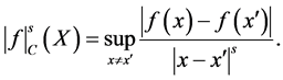
In this paper we concentrate on the non-identical setting that each sample is drawn according to a different distribution on Z. And each can also be decomposed to marginal distribution and conditional distribution. Assume they are elements of and respectively, where and are Hölder spaces with. Hölder spaces is the set of continuous functions with finite norm

where

We assume a polynomial convergence condition for both sequences and, i.e., there exist and, such that

(2)

(3)

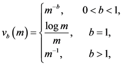
Power index b measures quantitatively differences between the non-identical setting and the i.i.d. case. The distributions are more similar as b is larger, and when it is indeed i.i.d. sampling, i.e. and for any. The following example is taken from [8] .

Example 1. Let be a sequence of bounded functions on X such that. Then the sequence defined by satisfies (2) for any.

On the other hand, most literature assume the output space is uniformly bounded, that is, for some positive constant M and almost surely with respect to. A typical kernel dependent result for the least-squares regularization algorithm under this assumption is [9] . There the authors get a learning rate close to 1 under some capacity condition for the hypothesis space. However, the most common distribution-Gaussian distribution is not bounded. This requirement is from the bounded condition in Bernstein inequality and limits the application of algorithms. In [10] - [13] , some unbounded conditions for the output space are discussed in different forms, which extends the classical bounded condition. Here we will follow the latter one which is more generalized and simple in expression, and this is the second novelty of this paper. We assume the moment incremental condition for the output space, an extension of that we proposed in [11] :

(4)

and

(5)

We can see the Gaussian distribution satisfies this setting.

Example 2. Let and. If for each and the condition distribution is a normal distribution with variance bounded by, then (4) is satisfied with and.

Next we need to introduce the covering number and interpolation space.

Definition 1. The covering number for a subset of and is defined to be the minimal integer N such that there exist N balls with radius covering.

Let the hypothesis space, be a compact Banach space with inclusion bounded and compact. We follow the assumption [14] [15] that there exist some constants and, such that the hypothesis space satisfies the capacity condition

(6)

where. Capacity condition describes the amount of functions in the hypothesis space.

The sample error will decrease but approximation error will increase when covering number of H is larger (or simply say H is larger). So how to choose an appropriate hypothesis space is the key problem of ERM algorithm. We will demonstrate this in our main theorem.

Definition 2. The interpolation space is a function space consists of with norm

where is the K-functional defined as

Interpolation space is used to characterize the position of the regression function, and it is related with the approximation error. Now we can state our main result as follow.

Theorem 1. If with bounded inclusion, and satisfies (6) with r, , for some, the sample distribution satisfies (2), (3) for some and, (4) and (5). For any, choose the hypothesis space to be the ball of H centered at 0 with radius, where and

Moreover, we assume all functions in H and are Hölder continuous of order s, i.e., there is a constant, such that

(7)

Then for any, with confidence at least, we have

Here is a constant independent with m and.

Remark 1. In [6] , the authors pointed out that if we choose the hypothesis space to be the reproducing kernel Hilbert space (RKHS) on, and the kernel, then our assumption (7) will hold true. In particular, if the kernel is chosen to be Gaussian kernel, then (7) holds for any. [16] discussed this in detail.

In all, we extend the polynomial convergence condition on the conditional distribution sequense and accordingly, set the moment inremental condition for the sequence in the least squares ERM algorithm. By error decomposition, truncate technique and unbounded concentration inequality, we can finally obtain the total error bound Theorem 1.

Compared with the non-identical settings in [6] and [17] , our setting is more general since the conditional distribution sequence is also a polynomially convergence sequence, but not identical as in their settings. This together with unbounded y lead to the main difficulty for the error analysis in this paper.

For the classical i.i.d. and bounded conditions, [9] indicates that and kernel while, the rate of least square regularization algorithm is for any. [17] shows that

under some conditions on kernel, object function, exponential convergence condition for distribution sequence and choose some special parameters, the optimal rate of online learning algorithm is close to

. In [6] , the best case occurs when and kernel. The rate of least square regularization algorithm can be close to. However, our result implicates that while,

tends to 1 and tends to 0, since p can be any integer, the learning rate can be arbitrarily close to, which is the same as in i.i.d. case [9] , and better than the former results with non-identical settings. With this result, we can extend the application of learning algorithm to more situations and still keep the best learning rate. The explicit expression of in the theorem can be found through the proof of the theorem below.

2. Error Decomposition

Our aim, the error is hard to bound directly, we need a transitional function for analyzing. By the compactness of and continuity of functional, we can denote

Then the generalization error can be written as

The first term on the right hand side is the sample error, and the second term is called approximation error which is independent with samples. [18] analyzed the approximation error by approxi- mation theory. In the following we mainly study the sample error bound.

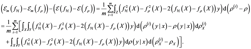
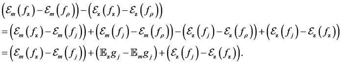
Now we break the sample error to some parts which can be bounded using truncate technique and unbounded concentration inequality. We refer the error decomposition to [6] . Denote

then and we have

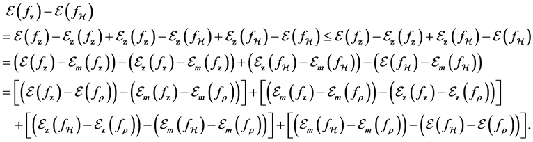
In the following, we call the first and fourth brackets drift errors, and the left sample errors. We will bound the two types of errors respectively in the following sections, and finally obtain the total error bounds.

3. Drift Errors

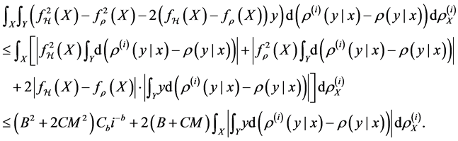
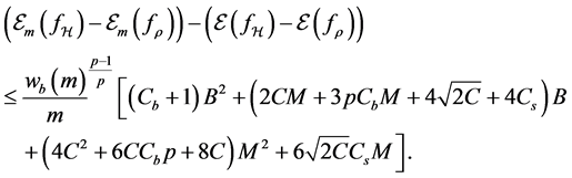
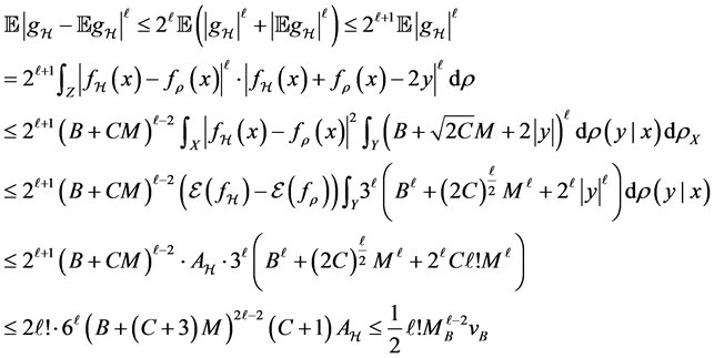
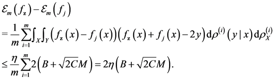
Firstly we consider the drift error involving in this section.To avoid handling two polynomial convergence sequences simultaneously, we break the drift errors to two parts. Meanwhile, a truncate technique is used to deal with the unbounded assumption. Since is a subset of, functions in is uniformly bounded. Then we have

Proposition 1. Assume for some, for any

Proof. From the definition of and, we know that

Since, we can bound the first term inside the bracket as follow.

But for any and, there holds

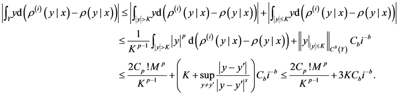
From (3.12) in [6] , we have

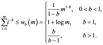
Then we can bound the sum of the first term as

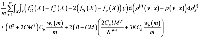
Choose K to be, we have

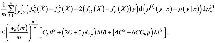
For the second term, notice, and so

Therefore

Combining the two bounds, we have

And this is indeed the proposition.

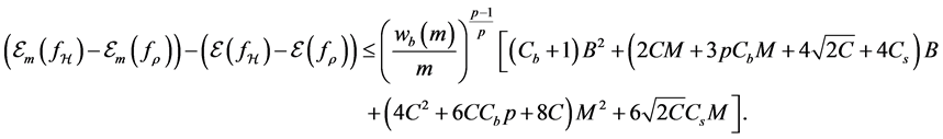
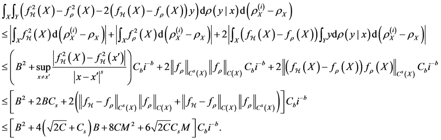
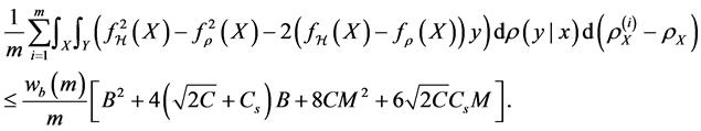
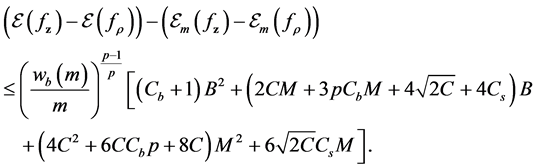
For the drift error involving, we have the same result since as well, i.e.,

Proposition 2. Assume 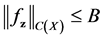for some, for any, we have

4. Sample Error Estimate

We devote this section to the analysis of the sample errors. For the sample error term involving, we will use the Bennett inequality as in [11] and [19] , which is initially introduced in [20] . Since two polynomial convergence conditions are posed on the marginal and conditional distribution sequences, we have to modify the

Bennett inequality to fit our setting. Denote and for an integrable function g, the lemma can be stated as follow.

Lemma 1. Assume holds for and some constants , then we have

For our non-identical setting, we can have a similar result from the same idea of proof. By denoting and, the following lemma holds.

Lemma 2. Assume and for some constants and any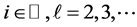, then we have

Now we can bound the sample error term by applying this lemma.

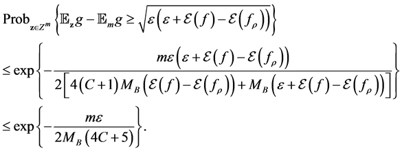
Proposition 3. Under the moment incremental condition (4), (5) and notations above, with probability at least, we have

where and is the approximation error.

Proof. Let

, then

Since, we have

for any, where 1and. In the same way, we have the following bounds

as well. Then from Lemma 2 above, we have

Set the right hand side to be, we can solve that

Therefore with confidence at least, there holds

This proves the proposition.

For the sample error term involving, analysis will be more involved since we need a concentration inequality for a set of functions. Firstly we have to introduce the ratio inequality [9] .

Lemma 3. Denote 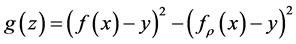for, which satisfies and for some constants and, then we have

Proof. Let to be in the Lemma 2, from the proof of the last proposition, we can conclude that

Note that and the lemma is proved.

Then we have the following result.

Lemma 4. For a set of functions with, construct functions 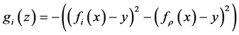for, with confidence at least, we have

where for any

Proof. Since is an element of, from Lemma 3 we have

then there holds

Set the right hand side to be and we have with probability at least,

Here. And this proves the lemma.

Now by a covering number argument we can bound the sample error term involving.

Proposition 4. If 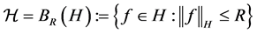for some, where H satisfies the capacity condition, for any, with confidence at least, there holds

Proof. Denote where is to be determined, then we can find an -net of, and there exist a function, we have

For the first term, since for all, we have

And for the third term,

we need to bound

Let and then

From Lemma 1 we have

Set the right hand side to be and with confidence at least we have

And this means,

with probability at least.

The second term can be bounded by 4 above. That is, with confidence at least, we have

Since by assumption, and

combining the three parts above, we have the following bound with confidence at least,

By choosing for balancing, we have

with confidence at least, this proves the proposition.

5. Approximation Error and Total Error

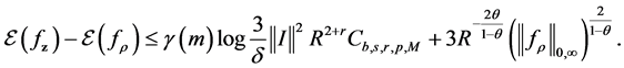
Combining the results above, we can derive the error bound for the generalization error.

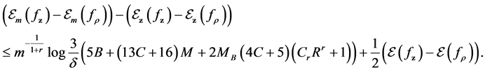
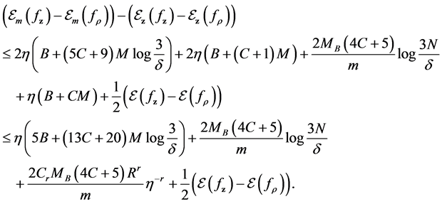
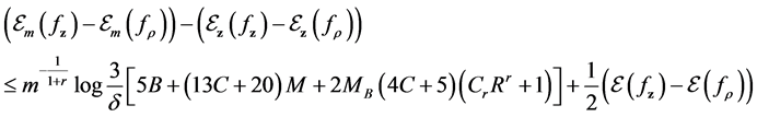
Proposition 5. Under the moment condition for the distribution of the sample and capacity condition for the hypothesis space, for any and, with confidence at least, we have

where.

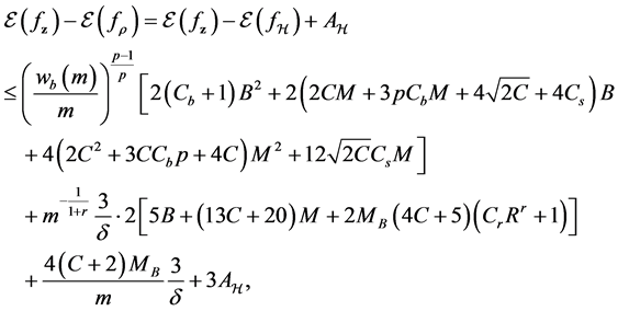
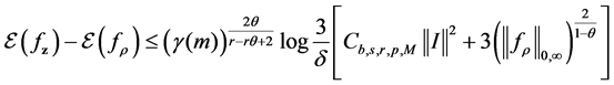
What is left to be determined in the proposition is the approximation error. By the choice of hypothesis space we can get our main result.

Proof of Theorem 1. Let

and, assume without loss of generality, and, Proposition 5 indicates that

holds with confidence at least for any, where is a constant independent on m or.

For the approximation error, we can bound it by Theorem 3.1 of [18] . Since the hypothesis space, and with, we have

The upper bound B is now chosen to be since, then with confidence at least,

By choosing

we have

holds with confidence at least. Denote, then the theorem is obtained.

6. Summary and Future Work

We investigate the least squares ERM algorithm with non-identical and unbounded sample, i.e., polynomial convergence for and and moment inremental condition for the latter ones. Analogue

error decomposition as classical analysis for least sqaures regularization [9] [11] is conducted. Truncate techni- que is introduced for handling unbounded setting, and Bennett concentration inequality is used for the sample error. By the above analysis we finally get the error bound and learning rate.

However, our work only considers the ERM algorithm. It is neccesary for us to extend this to the regulari- zation algorithms which are more widely used in practice. A more recent relative reference can be found in [21] . Another interesting topic in future study is dependent sampling [7] .

Cite this paper

Weilin Nie,Cheng Wang, (2016) Error Analysis of ERM Algorithm with Unbounded and Non-Identical Sampling. Journal of Applied Mathematics and Physics,04,156-168. doi: 10.4236/jamp.2016.41019

References

NOTES

^*This work is supported by NSF of China (Grant No. 11326096, 11401247), Foundation for Distinguished Young Talents in Higher Education of Guangdong, China (No. 2013LYM 0089), Doctor Grants of Huizhou University (Grant No. C511.0206) and NSF of Guangdong Province in China (No. 2015A030313674).

^#Corresponding author.

References

- 1. Cucker, F. and Zhou, D.X. (2007) Learning Theory: An Approximation Theory Viewpoint. Cambridge University Press, Cambridge.
http://dx.doi.org/10.1017/CBO9780511618796 - 2. Cucker, F. and Smale, S. (2002) On the Mathematical Foundations of Learning. Bulletin of the American Mathematical Society, 39, 1-49.
- 3. Dehling, H., Mikosch, T. and Sorensen, M. (2002) Empirical Process Techniques for Dependent Data. Birkhauser Boston, Inc., Boston.
http://dx.doi.org/10.1007/978-1-4612-0099-4 - 4. Steinwart, I., Hush, D. and Scovel, C. (2009) Learning from Dependent Observations. Journal of Multivariate Analysis, 100, 175-194.
- 5. Steinwart, I. and Christmann, A. (2009) Fast Learning from Non-i.i.d. Observations. In: Bengio, Y., Schuurmans, D., Lafferty, J.D., Williams, C.K.I. and Culotta, A., Eds., Advances in Neural Information Processing Systems 22, Curran and Associates, Inc., Yellowknife, 1768-1776.
- 6. Xiao, Q.W. and Pan, Z.W. (2010) Learning from Non-Identical Sampling for Classification. Advances in Computational Mathematics, 33, 97-112.
- 7. Pan, Z.W. and Xiao, Q.W. (2009) Least-Square Regularized Regression with Non-i.i.d. Sampling. Journal of Statistical Planning and Inference, 139, 3579-3587.
- 8. Hu, T. and Zhou, D.X. (2009) Online Learning with Samples Drawn from Non-identical Distributions. Journal of Machine Learning Research, 10, 2873-2898.
- 9. Wu, Q., Ying, Y. and Zhou, D.X. (2006) Learning Rates of Least-Square Regularized Regression. Foundations of Computational Mathematics, 6, 171-192.
- 10. Capponnetto, A. and De Vito, E. (2007) Optimal Rates for the Regularized Least Squares Algorithm. Foundations of Computational Mathematics, 7, 331-368.
- 11. Wang, C. and Zhou, D.X. (2011) Optimal Learning Rates for Least Squares Regularized Regression with Unbounded Sampling. Journal of Complexity, 27, 55-67.
- 12. Guo, Z.C. and Zhou, D.X. (2013) Concentration Estimates for Learning with Unbounded Sampling. Advances in Computational Mathematics, 38, 207-223.
- 13. He, F. (2014) Optimal Convergence Rates of High Order Parzen Windows with Unbounded Sampling. Statistics & Probability Letters, 92, 26-32.
- 14. Zhou, D.X. (2002) The Covering Number in Learning Theory. Journal of Complexity, 18, 739-767.
- 15. Zhou, D.X. (2003) Capacity of Reproducing Kernel Spaces in Learning Theory. IEEE Transactions on Information Theory, 49, 1743-1752.
- 16. Zhou, D.X. (2008) Derivative Reproducing Properties for Kernel Methods in Learning Theory. Journal of Computational and Applied Mathematics, 220, 456-463.
- 17. Smale, S. and Zhou, D.X. (2009) Online Learning with Markov Sampling. Analysis and Applications, 7, 87-113.
- 18. Smale, S. and Zhou, D.X. (2003) Estimating the Approximation Error in Learning Theory. Analysis and Applications, 1, 17-41.
- 19. Wang, C. and Guo, Z.C. (2012) ERM Learning with Unbounded Sampling. Acta Mathematica Sinica, English Series, 28, 97-104.
- 20. Bennett, G. (1962) Probability Inequalities for the Sum of Independent Random Variables. Journal of the American Statistical Association, 57, 33-45.
- 21. Cai, J. (2013) Coefficient-Based Regression with Non-Identical Unbounded Sampling. Abstract and Applied Analysis, 2013, Article ID: 134727.
http://dx.doi.org/10.1155/2013/134727