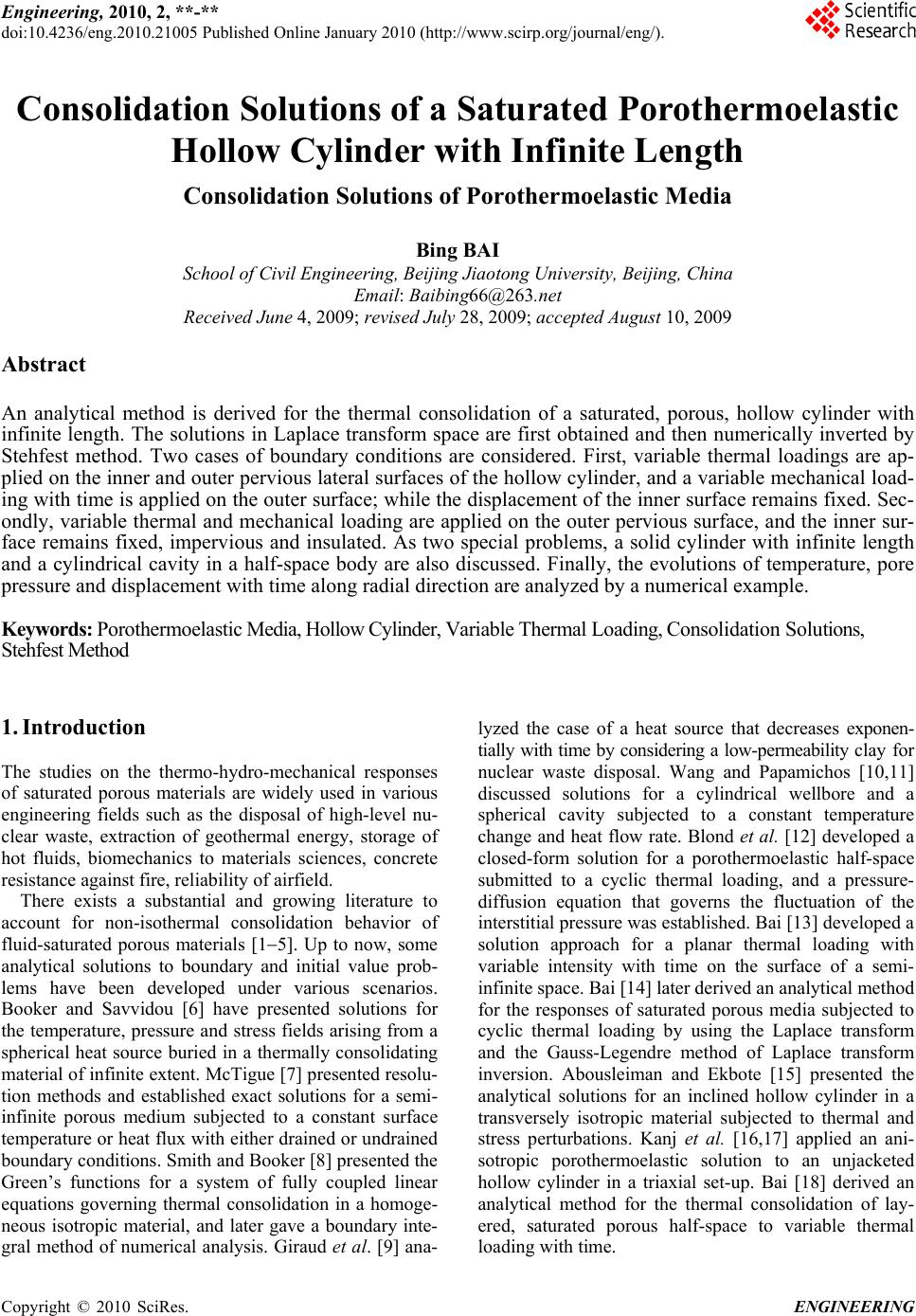Engineering, 2010, 2, **-**
doi:10.4236/eng.2010.21005 Published Online January 2010 (http://www.scirp.org/journal/eng/).
Consolidation Solutions of a Saturated Porothermoelastic
Hollow Cylinder with Infinite Length
Consolidation Solutions of Porothermoelastic Media
Bing BAI
School of Civil Engineering, Beijing Jiaotong University, Beijing, China
Received June 4, 2009; revised July 28, 2009; accepted August 10, 2009
Abstract
An analytical method is derived for the thermal consolidation of a saturated, porous, hollow cylinder with
infinite length. The solutions in Laplace transform space are first obtained and then numerically inverted by
Stehfest method. Two cases of boundary conditions are considered. First, variable thermal loadings are ap-
plied on the inner and outer pervious lateral surfaces of the hollow cylinder, and a variable mechanical load-
ing with time is applied on the outer surface; while the displacement of the inner surface remains fixed. Sec-
ondly, variable thermal and mechanical loading are applied on the outer pervious surface, and the inner sur-
face remains fixed, impervious and insulated. As two special problems, a solid cylinder with infinite length
and a cylindrical cavity in a half-space body are also discussed. Finally, the evolutions of temperature, pore
pressure and displacement with time along radial direction are analyzed by a numerical example.
Keywords: Porothermoelastic Media, Hollow Cylinder, Variable Thermal Loading, Consolidation Solutions,
Stehfest Method
1. Introduction
The studies on the thermo-hydro-mechanical responses
of saturated porous materials are widely used in various
engineering fields such as the disposal of high-level nu-
clear waste, extraction of geothermal energy, storage of
hot fluids, biomechanics to materials sciences, concrete
resistance against fire, reliability of airfield.
There exists a substantial and growing literature to
account for non-isothermal consolidation behavior of
fluid-saturated porous materials [15]. Up to now, some
analytical solutions to boundary and initial value prob-
lems have been developed under various scenarios.
Booker and Savvidou [6] have presented solutions for
the temperature, pressure and stress fields arising from a
spherical heat source buried in a thermally consolidating
material of infinite extent. McTigue [7] presented resolu-
tion methods and established exact solutions for a semi-
infinite porous medium subjected to a constant surface
temperature or heat flux with either drained or undrained
boundary conditions. Smith and Booker [8] presented the
Green’s functions for a system of fully coupled linear
equations governing thermal consolidation in a homoge-
neous isotropic material, and later gave a boundary inte-
gral method of numerical analysis. Giraud et al. [9] ana-
lyzed the case of a heat source that decreases exponen-
tially with time by considering a low-permeability clay for
nuclear waste disposal. Wang and Papamichos [10,11]
discussed solutions for a cylindrical wellbore and a
spherical cavity subjected to a constant temperature
change and heat flow rate. Blond et al. [12] developed a
closed-form solution for a porothermoelastic half-space
submitted to a cyclic thermal loading, and a pressure-
diffusion equation that governs the fluctuation of the
interstitial pressure was established. Bai [13] developed a
solution approach for a planar thermal loading with
variable intensity with time on the surface of a semi-
infinite space. Bai [14] later derived an analytical method
for the responses of saturated porous media subjected to
cyclic thermal loading by using the Laplace transform
and the Gauss-Legendre method of Laplace transform
inversion. Abousleiman and Ekbote [15] presented the
analytical solutions for an inclined hollow cylinder in a
transversely isotropic material subjected to thermal and
stress perturbations. Kanj et al. [16,17] applied an ani-
sotropic porothermoelastic solution to an unjacketed
hollow cylinder in a triaxial set-up. Bai [18] derived an
analytical method for the thermal consolidation of lay-
ered, saturated porous half-space to variable thermal
loading with time.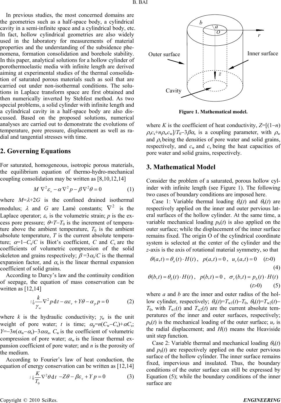

B. BAI
In previous studies, the most concerned domains are
the geometries such as a half-space body, a cylindrical
cavity in a semi-infinite space and a cylindrical body, etc.
In fact, hollow cylindrical geometries are also widely
used in the laboratory for measurements of material
properties and the understanding of the subsidence phe-
nomena, formation consolidation and borehole stability.
In this paper, analytical solutions for a hollow cylinder of
porothermoelastic media with infinite length are derived
aiming at experimental studies of the thermal consolida-
tion of saturated porous materials such as soil that are
carried out under non-isothermal conditions. The solu-
tions in Laplace transform space are first obtained and
then numerically inverted by Stehfest method. As two
special problems, a solid cylinder with infinite length and
a cylindrical cavity in a half-space body are also dis-
cussed. Based on the proposed solutions, numerical
analyses are carried out to demonstrate the evolutions of
temperature, pore pressure, displacement as well as ra-
dial and tangential stresses with time.
2. Governing Equations
For saturated, homogeneous, isotropic porous materials,
the equilibrium equation of thermo-hydro-mechanical
coupling consolidation may be written as [8,10,12,14]
0
222 
 pM v (1)
where M=  +2G is the confined drained isothermal
modulus;  and G are Lamé constants; is the
Laplace operator; 
v is the volumetric strain; p is the ex-
cess pore pressure;
 =TT0 is the increment of tempera-
ture above the ambient temperature, T0 is the ambient
absolute temperature, T is the current absolute tempera-
ture;
 =1Cs/C is Biot’s coefficient, C and Cs are the
coefficients of volumetric compression of the solid
skeleton and grains respectively;
 =3 
s/C is the thermal
expansion factor, and

s is the linear thermal expansion
coefficient of solid grains.
2

According to Darcy’s law and the continuity condition
of seepage, the equation of mass conservation can be
written as [12,14]
0d
0
2
pYtp
k
pv
t
w


(2)
where k is the hydraulic conductivity;

w is the unit
weight of pore water; t is time;

p=n(CwCs)+
 Cs;
Y=3n(

w

s)3

s, Cw is the coefficient of volumetric
compression of pore water;

w is the linear thermal ex-
pansion coefficient of pore water; and n is the porosity of
the medium.
According to Fourier’s law of heat conduction, the
equation of energy conservation can be written as [12,14]

tt
T
K
0
2
0
d 
0

pYZ v



(3)
z
r
a
O
Outer surface
b
Cavity
Inner surface
Figure 1. Mathematical model.
where K is the coefficient of heat conductivity, Z=[(1n)

scs+n

wcw]/T03

s is a coupling parameter, with

w
and 
s being the densities of pore water and solid grains,
respectively, and cw and cs being the heat capacities of
pore water and solid grains, respectively.
3. Mathematical Model
Consider the problem of a saturated, porous hollow cyl-
inder with infinite length (see Figure 1). The following
two cases of boundary conditions are imposed here.
Case 1: Variable thermal loading

a(t) and

b(t) are
respectively applied on the inner and outer pervious lat-
eral surfaces of the hollow cylinder. At the same time, a
variable mechanical loading pb(t) is also applied on the
outer surface; while the displacement of the inner surface
remains fixed. The origin O of the cylindrical coordinate
system is selected at the center of the cylinder and the
z-axis is the axis of rotational material symmetry, so that
)()(),( tHtta a




, , (t0) 0),( tap 0),( taur
(4)
)()(),(tHttb b




, , 0),(tbp )()(),( tHtptb br



(t0) (5)
where a and b are the inner and outer radius of the hol-
low cylinder, respectively; 
a(t)=Tw1(t)T0,

b(t)=Tw2(t)
T0, with Tw1(t) and Tw2(t) are the current absolute tem-
peratures of the inner and outer surfaces, respectively;
pb(t) is the mechanical loading of the outer surface; ur is
the radial displacement; and H(t) means the Heaviside
unit step function.
Case 2: Variable thermal and mechanical loading 
b(t)
and pb(t) are respectively applied on the outer pervious
surface of the hollow cylinder. The inner surface remains
fixed, impervious and insulated. Thus, the boundary
conditions of the outer surface can still be expressed by
Equation (5); while the boundary conditions of the inner
surface are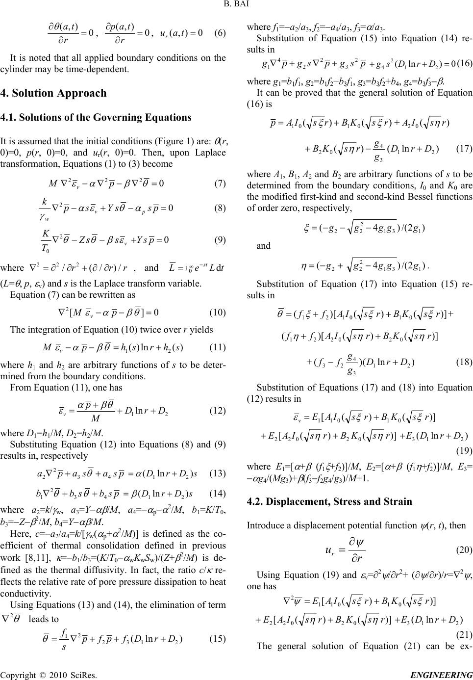

B. BAI
0
),( 


r
ta

, 0
),( 


r
tap , 0),(

taur (6)
It is noted that all applied boundary conditions on the
cylinder may be time-dependent.
4. Solution Approach
4.1. Solutions of the Governing Equations
It is assumed that the initial conditions (Figure 1) are:  (r,
0)=0, p(r, 0)=0, and ur(r, 0)=0. Then, upon Laplace
transformation, Equations (1) to (3) become
0
222 
 pM v (7)
0
2 pssYsp
k
pv
w


(8)
v
ssZ
T
K
 2
0
0 psY (9)
where , and
222
/(/)/rr r 0dtLeL st
(L=
 , p, 
v) and s is the Laplace transform variable.
Equation (7) can be rewritten as
0][
2
 pM v (10)
The integration of Equation (10) twice over r yields
)(ln)( 21 shrshpM v  (11)
where h1 and h2 are arbitrary functions of s to be deter-
mined from the boundary conditions.
From Equation (11), one has
21ln DrD
M
p
v




(12)
where D1=h1/M, D2=h2/M.
Substituting Equation (12) into Equations (8) and (9)
results in, respectively
psasapa43
2
2
 sDrD )ln(21 

(13)
psbsbb 43
2
1
 sDrD )ln( 21 


(14)
where a2=k/ 
w, a3=Y
 /M, a4= 
p

2/M, b1=K/T0,
b3=Z 
2/M, b4=Y
 /M.
Here, c=a2/a4=k/[ 
w(

p+

2/M)] is defined as the co-
efficient of thermal consolidation defined in previous
work [8,11],  =b1/b3=(K/T0 
wKwSw)/(Z+

2/M) is de-
fined as the thermal diffusivity. In fact, the ratio c/  re-
flects the relative rate of pore pressure dissipation to heat
conductivity.
Using Equations (13) and (14), the elimination of term

2
 leads to
)ln( 2132
2
1DrDfpfp
s
f
 (15)
where f1=a2/a3, f2=a4/a3, f3=  /a3.
Substitution of Equation (15) into Equation (14) re-
sults in
psgpsgpg 2
3
2
2
4
1 0)ln(21
2
4 DrDsg (16)
where g1=b1f1, g2=b1f2+b3f1, g3=b3f2+b4, g4=b3f3
 .
It can be proved that the general solution of Equation
(16) is
)()(0101rsKBrsIAp   +)(
02 rsIA

)ln()(21
3
4
02 DrD
g
g
rsKB  (17)
where A1, B1, A2 and B2 are arbitrary functions of s to be
determined from the boundary conditions, I0 and K0 are
the modified first-kind and second-kind Bessel functions
of order zero, respectively,
)2/()4( 131
2
22 ggggg 

and



2
(g

)2/()4 131
2
2gggg .
Substitution of Equation (17) into Equation (15) re-
sults in
)]()()[( 010121 rsKBrsIAff   +
)]()()[( 020221 rsKBrsIAff  
+)ln()(21
3
4
23 DrD
g
g
ff  (18)
Substitution of Equations (17) and (18) into Equation
(12) results in
)]()([ 01011rsKBrsIAE
v
 
)]()([02022 rsKBrsIAE   )ln( 213 DrDE


(19)
where E1=[
 +  (f1  +f2)]/M, E2=[  +  (f1  +f2)]/M, E3=

 g4/(Mg3)+  (f3f2g4/g3)/M+1.
4.2. Displacement, Stress and Strain
Introduce a displacement potential function
 (r, t), then
r
ur




(20)
Using Equation (19) and 
v=2
 /r2+ (  /r)/r=2  ,
one has
)]()([01011
2rsKBrsIAE
 
)]()([02022 rsKBrsIAE   )ln( 213 DrDE


(21)
The general solution of Equation (21) can be ex-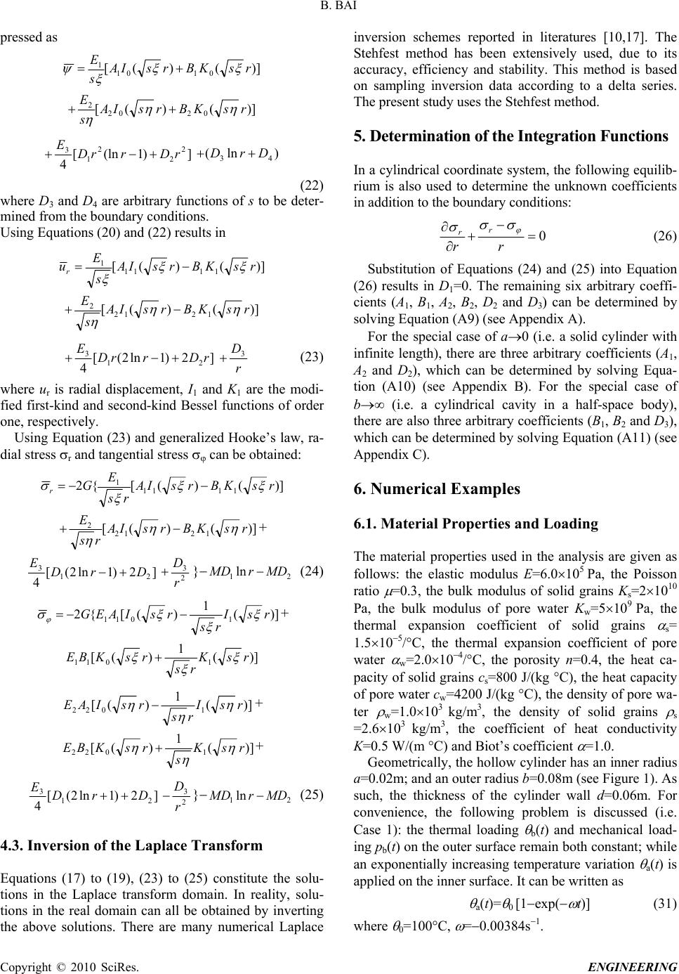

B. BAI
pressed as
)]()([ 0101
1rsKBrsIA
s
E


 
)]()([ 0202
2rsKBrsIA
s
E



])1(ln[
4
2
2
2
1
3rDrrD
E )ln(43 DrD 
(22)
where D3 and D4 are arbitrary functions of s to be deter-
mined from the boundary conditions.
Using Equations (20) and (22) results in
)]()([ 1111
1rsKBrsIA
s
E
ur 


)]()([ 1212
2rsKBrsIA
s
E



]2)1ln2([
421
3rDrrD
E
r
D3
 (23)
where ur is radial displacement, I1 and K1 are the modi-
fied first-kind and second-kind Bessel functions of order
one, respectively.
Using Equation (23) and generalized Hooke’s law, ra-
dial stress r and tangential stress  can be obtained:
)]()([{2 1111
1rsKBrsIA
rs
E
G
r


 
)]()([ 1212
2rsKBrsIA
rs
E


 +
]2)1ln2([
421
3DrD
E 2
3
r
D
} (24)
21ln MDrMD 
)](
1
)([{2 1011 rsI
rs
rsIAEG 



 +
)](
1
)([ 1011 rsK
rs
rsKBE 

 
)](
1
)([1022 rsI
rs
rsIAE 

 +
)](
1
)([ 1022rsK
s
rsKBE 

 +
]2)1ln2([
421
3DrD
E 2
3
r
D
} (25)
21ln MDrMD 
4.3. Inversion of the Laplace Transform
Equations (17) to (19), (23) to (25) constitute the solu-
tions in the Laplace transform domain. In reality, solu-
tions in the real domain can all be obtained by inverting
inversion schemes reported in literatures [10,17]. The
Stehfest method has been extensively used, due to its
accuracy, efficiency and stability. This method is based
on sampling inversion data according to a delta series.
The present study uses the Stehfest method.
the above solutions. There are many numerical Laplace
. Determination of the Integration Functions
a cylindrical coordinate system, the following equilib-
5
In
rium is also used to determine the unknown coefficients
in addition to the boundary conditions:
0

r




rr
r (26)
Substitution of Equations (24) and (25) into Equation
(2
cylinder with
in
. Numerical Examples
.1. Material Properties and Loading
he material properties used in the analysis are given as
ner radius
a=
(31)
where 
0=100C,
 =
6) results in D1=0. The remaining six arbitrary coeffi-
cients (A1, B1, A2, B2, D2 and D3) can be determined by
solving Equation (A9) (see Appendix A).
For the special case of a0 (i.e. a solid
finite length), there are three arbitrary coefficients (A1,
A2 and D
2), which can be determined by solving Equa-
tion (A10) (see Appendix B). For the special case of
b (i.e. a cylindrical cavity in a half-space body),
there are also three arbitrary coefficients (B1, B2 and D3),
which can be determined by solving Equation (A11) (see
Appendix C).
6
6
T
follows: the elastic modulus E=6.0105 Pa, the Poisson
ratio
 =0.3, the bulk modulus of solid grains Ks=21010
Pa, the bulk modulus of pore water Kw=5109 Pa, the
thermal expansion coefficient of solid grains

s=
1.5105/C, the thermal expansion coefficient of pore
water

w=2.0104/C, the porosity n=0.4, the heat ca-
pacity of solid grains cs=800 J/(kg C), the heat capacity
of pore water cw=4200 J/(kg C), the density of pore wa-
ter 
w=1.0103 kg/m3, the density of solid grains

s
=2.6103 kg/m3, the coefficient of heat conductivity
K=0.5 W/(m C) and Biot’s coefficient
 =1.0.
Geometrically, the hollow cylinder has an in
0.02m; and an outer radius b=0.08m (see Figure 1). As
such, the thickness of the cylinder wall d=0.06m. For
convenience, the following problem is discussed (i.e.
Case 1): the thermal loading 
b(t) and mechanical load-
ing pb(t) on the outer surface remain both constant; while
an exponentially increasing temperature variation

a(t) is
applied on the inner surface. It can be written as

a(t)=

0 [1exp(
 t)]
0.00384s1.

B. BAI
0.0
0.2
0.4
0.6
0.8
1.0
0.0 0.20.4 0.60.8 1.0
0.1
0.4
1
2
10
r
/b



0
T=
Figure 2. Distributions of temperature along radial distance.
-5000
-4000
-3000
-2000
-1000
0
0.0 0.2 0.40.6 0.8 1.0
0.1
0.4
1
2
10
5000
4000
3000
2000
1000
0
r
/b
p (Pa)
T=
Figure 3. Pore pressure varying with T under therma
.2. Responses under Thermal Loading
this section, we assume that the thermal loading
t
he elapsed
tim
igure 3 that at early times (e.g.
T=
l
loading.
6
In

b(t)=0, and the mechanical loading p b(t)=0; while the
hermal loading given by Equation (31) is applied on the
inner surface. A dimensionless time is defined as T=  t/b2
(i.e. time factor). Figures 2 to 6 present respectively the
temperature, pore pressure, radial displacement, radial
stress and tangential stress distributions along radial dis-
tance for various time factors (e.g. T=0.1, 0.4, 1, 2, 10,
i.e. t=3.9, 15.6, 39.0, 78.1, 390.4min; c/  =1).
It can be seen from Figure 2 that, with t
e, the temperature is gradually conducted from the
inner surface of the hollow cylinder to the points away
from the surface. As the time factor T increases continu-
ously (e.g. T=10), the temperature values finally reach a
quasi-steady state. At this time, the temperature distribu-
tion along the radial distance remains a steady tempera-
ture gradient. Certainly, the values of temperature gradi-
ent near the inner surface (e.g. r/b=0.250.4) are greater
than those of the points in the vicinity of the outer sur-
face (e.g. r/b=0.81.0).
It can be seen from F
0.1, 0.4) the pore pressure value in the vicinity of the
0
.00008
0
.00006
0
.00004
0
.00002
0
.00000
0
.00002
0
.00004 4
2
0
2
4
6
8
00.2 0.4 0.6 0.81
0.1
0.4
1
2
10
r
/b
u
r
/d
T
=
Figure 4. Radial displacement varying with T under ther-
mal loading.
-600
-500
-400
-300
-200
-100
0
100
200
300
00.2 0.4 0.6 0.81
0.1
0.4
1
2
10
300
200
100
0
100
200
300
400
500
600
r
/b 
r
(Pa)
T
=
Figure 5. Radial stress varying with T under thermal loading
inner surface takes on a rising trend, and then is con-
di
6, in the whole processes
of
.
ducted from the inner surface of hollow cylinder to the
outer surface; while the peak value gradually moves to
the outer surface. At later times (e.g. T=2, 10), the pore
pressure begins to decrease quickly due to the com-
pletely pervious lateral surfaces of the hollow cylinder,
and finally is dissipated to zero along the radial distance.
Figure 4 shows that, at early times (e.g. T=0.1) the ra-
al displacement takes on an expanding trend (i.e. nega-
tive displacement) along the whole radial distance; how-
ever with time factor T increasing (e.g. T=0.4, 1, 2), the
radial displacements of the points in the vicinity of the
inner surface begin to contract (i.e. positive displacement)
due to the strong coupling between the expansion of
grains and the drainage of pore water. With the succes-
sive dissipation of pore pressure (e.g. T=10), the radial
displacement eventually takes an increasing trend with
the radial distance increasing.
As shown in Figures 5 and
consolidation, the radial and tangential stress distribu-
tions are very complicated due to the coupling effects of
pore pressure dissipation and thermal stress. In fact, at
early times (e.g. T=0.1, 0.4, 1) the radial stress in the
vicinity of the inner surface begins to increase (being
negative values, i.e. stretching stress), then (e.g. T=2)
decreases with time factor increasing, and finally (e.g.

B. BAI
-5000
-4000
-3000
-2000
-1000
0
1000
2000 2000
00.2 0.40.6 0.81
0.1
0.4
1
2
10
1000
0
1000
2000
3000
4000
5000
r
/b


(Pa)
T=
Figure 6. Tangential stress varying with T under thermal
loading.
0.0
0.2
0.4
0.6
0.8
1.0
0.0 0.2 0.4 0.6 0.8 1.0
0.1
0.4
1
2
10
r
/b



0
T
=
Figure 7. Distributions of temperature along radial distanc
=10) takes on a positive value (i.e. compressive stress).
.3. Responses under Thermal and Mechanical
he responses of the porothermoelastic hollow cylinder
n from Figure 7 that the developing trend
of
e
(c/k=1).
T
On the other hand, the tangential stress in the middle part
of the wall of the hollow cylinder initially takes a com-
pressive state (i.e. positive value), and eventually pre-
sents a stretching state (i.e. negative value).
6
Loading
T
under thermo-hydro-mechanical coupling are discussed
in this section. Here, the thermal loading

b(t)=20C, and
the mechanical loading pb(t)=100kPa; while the thermal
loading given by Equation (31) is applied on the inner
surface. Figures 7 to 11 present respectively the tem-
perature, pore pressure, radial displacement, radial stress
and tangential stress distributions as a function of the
radial distance for various time factors (e.g. T=0.1, 0.4, 1,
2, 10; c/  =1).
It can be see
the temperature along the radial distance is similar to
the temperature distributions in Figure 2 except for the
values on the outer surface of the hollow cylinder, which
0.0
0.2
0.4
0.6
0.8
1.0
T
0.1
0.4
1
0.0 0.20.4 0.60.8 1.0
2
/
p
0
p
10
r
/b
=
Figure 8. Distributions of pore pressure along radial dis-
tance (c/k=1).
-0.07
-0.06
-0.05
-0.04
-0.03
-0.02
-0.01
0.00
0.0 0.2 0.40.60.8 1.0
0.07
0.06
0.05
0.04
0.03
0.02
0.01
0
0.1
0.4
1
2
10
r
/b
T=
u
r
/d
Figure 9. Distributions of radial displacement along radia
is due to the difference of boundary thermal loading.
,
th
ent anywhere
in
l
distance (c/k=1).
Calculation results for various c/  (e.g. c/  =0.1, 1, 2)
show that the coupling effects of displacement and stress
fields on temperature field can be generally neglected.
By virtue of the imposed lateral boundary conditions
e pore pressure drops almost instantaneously at the
inner and outer boundaries (i.e. r=a and r=b) as indicated
in Figure 8. As such, there exists a peak value of pore
pressure in the inner layers. As time progresses, the pore
pressure peak value gradually diffuses and flattens. It
should be noted that the pore pressure in the vicinity of
the outer boundary seems to dissipate more quickly,
which is due to the greater drainage surface of the outer
boundary than that of the inner boundary.
Figure 9 shows that the radial displacem
the cylinder contracts (i.e. being positive value) with
the diffusion of the pore water. However, it is noticed
that, at early times (e.g. T=0.1, 0.4), the radial displace-
ment in the local range of the wall (e.g. 0.4r/b0.9) is
even smaller than that in the vicinity of the inner bound-
ary (here, noting ur(a, t)=0). This may be attributed to the

B. BAI
0.7
0.8
0.9
1.0
1.1
0.0 0.2 0.40.6 0.8 1.0
0.1
0.4
1
2
10
r
/b

r
/p
b
T
=
Figure 10. Distributions of radial stresses along radial dis-
consolidation deformation (i.e. shrinkage of the cylinder)
om Figure 10 that the evolution of radial
st
n at
ea
. Conclusions
) An analytical method is derived for the thermal con-
elastic hollow cylin-
de
tance (c/k=1).
caused by the rapid dissipation in the vicinity of the per-
vious inner and outer surfaces. Obviously, this phe-
nomenon vanishes as time progresses (see Figure 9).
Furthermore, the radial displacement ur will take on a
linear relation with radial distance r at time factor T
tends to infinity.
It can be seen fr
ress is very complicated. At early times (e.g. T=0.1, 0.4),
the radial stress in the local range of the wall (e.g.
0.3r/b0.4) is even greater than the applied mechanical
loading pb on the outer surface (i.e. 
r/pb1). Obviously, as
time factor T increases, the radial stress takes on a mono-
tonically increasing trend with radial distance, and finally
reach a steady state at time factor T tends to infinity.
Figure 11 presents a tangential stress concentratio
ch of the boundaries of the cylinder. These stresses are
generated as a result of the hoop effects that accompany
the inner and outer diffusion fronts. Moreover, this stress
concentration is more severe at early times. With diffu-
sion, the tangential stress concentrations at the lateral
surfaces weaken and diminish in magnitude while higher
compressive tangential stresses ( 
/pb1) are noted to
form inside the cylinder.
7
1
solidation of a saturated, porous, hollow cylinder with
infinite length. The solutions in Laplace transform space
are first obtained and then numerically inverted by
Stehfest method. As two special problems, a solid cylin-
der with infinite length and a cylindrical cavity in a
half-space body are also discussed.
2) The responses of a porothermo
r subjected to exponentially increasing thermal loading
with time on the inner surface are discussed. Calculations
show that, as the temperature is gradually conducted from
the inner surface to the points away from the surface,
0.8
1.0
1.2
1.4
1.6


/p
b
0.1
T
0.4
1
2
10
0.0 0.20.4 0.60.8 1.0
r
/b
=
Figure 11. Distributions of tangential stresses along radial
the pore pressure value initially takes on a rising trend,
cylin-
de
. Acknowledgements
inancial support from the National Natural Science
. References
] M. Kurashige, “A thermoelastic theory of fluid-filled
for an
nd J. R.
distance (c/k=1).
and then begins to decrease quickly due to the pervious
lateral surfaces. In addition, the radial displacement ini-
tially increases with the increase of temperature and then
contracts with the diffusion of pore water, which is due
to the strong coupling effects of the expansion of grains,
the drainage of pore water, and the radial and tangential
stress varying with time under thermal loading.
3) The responses of a porothermoelastic hollow
r under thermo-hydro-mechanical coupling have also
been analyzed. Numerical results indicate that the tem-
perature difference generates both pore pressure and
stress distributions in the cylinder. A pore pressure field,
as well as a radial displacement, a radial and tangential
stress fields, are created as a result of the compaction of
the cylinder and the heating of the borehole wall. Corre-
spondingly, this results in the complicated evolution
processes of all the variables, and can be explained by
the consolidation deformation due to the thermal stress
and the rapid dissipation of pore pressure in the vicinity
of the pervious inner and outer surfaces.
8
F
Foundation of China (NSFC) under approved grant No.
50879003 is gratefully acknowledged.
9
[1
porous materials,” International Journal of Solids and
Structures, Vol. 25, No. 9, pp. 10391052, 1989.
[2] X. Li, “A generalized theory of thermoelasticity
anisotropic medium,” International Journal of Engineer-
ing Science, Vol. 30, No. 5, pp. 571577, 1992.
[3] H. N. Seneviratne, J. P. Carter, D. W. Airey, a
Booker, “A review of models for predicting the ther-

B. BAI
tic cou-
nd ther-
po
n’s function for a
oelastic
ternational Journal for
ational
al loading on the surface of semi-infinite
s media
hermoelastic transversely iso-
n-
nterna-
o variable thermal loading,” Applied Mathemat-
ics and Mechanics, Vol. 27, No. 11, pp. 15311539,
2006.
momechanical behavior of soft clays,” International
Journal for Numerical and Analytical Methods in Ge-
omechanics, Vol. 17, No. 10, pp. 715733,1993.
[4] M. Bai and Y. Abousleiman, “Thermoporoelas
pling with application to consolidation,” International
Journal for Numerical and Analytical Methods in Ge-
omechanics, Vol. 21, No. 2, pp. 121132, 1997.
[5] R. W. Zimmerman, “Coupling in poroelasticity a
moelasticity,” International Journal of Rock Mechanics
and Mining Sciences, Vol. 37, No. 1, pp. 7987, 2000.
[6] J. R. Booker and C. Savvidou, “Consolidation around a sp
spherical heat source,” International Journal of Solids and
Structures, Vol. 20, No. 5, pp. 10791090, 1984.
[7] D. F. McTigue, “Flow to a heated borehole in rous, subjected to cyclic thermal loading,” Computers and
Geotechnics, Vol. 33, No. 4, pp. 396403, 2006.
[15] Y. Abousleiman and S. Ekbote, “Solutions for the in-
clined borehole in a porot
thermoelastic rock: Analysis,” Water Resources Research,
Vol. 26, No. 8, pp. 17631774, 1990.
[8] D. W. Smith and J. R. Booker, “Gree
fully coupled thermoporoelastic materials,” International
Journal for Numerical and Analytical Methods in Ge-
omechanics, Vol. 17, No. 2, pp. 139163, 1993.
[9] A. Giraud, F. Homand, and G. Rousset, “Therm ics o
and thermoplastic response of a double-layer porous
space containing a decaying heat source,” International
Journal for Numerical and Analytical Methods in Ge-
omechanics, Vol. 22, No. 2, pp. 133149, 1998.
[10] Y. Wang and E. Papamichos, “An analytical solution for
tional Journal for Numerical and Analytical Methods in
Geomechanics, Vol. 29, No. 1, pp. 103126, 2005.
[18] B. Bai, “Thermal consolidation of layered porous half-
space t
conductive heat flow and the thermally induced fluid
flow around a wellbore in a poroelastic medium,” Water
Resource Research, Vol. 36, No. 5, pp. 33753384, 1994.
[11] Y. Wang and E. Papamichos, “Thermal effects on fluid
flow and hydraulic fracturing from wellbores and cavities
in low-permeability formations,” In
Numerical and Analytical Methods in Geomechanics, Vol.
23, No. 15, pp. 18191834, 1999.
[12] E. Blond, N. Schmitt, and F. Hild, “Response of saturated
porous media to cyclic thermal loading,” Intern
Journal for Numerical and Analytical Methods in Ge-
omechanics, Vol. 27, No. 11, pp. 883904, 2003.
[13] B. Bai, “Response of saturated porous media subjected to
local therm
ace,” Acta Mechanica Sinica, Vol. 22, No. 1, pp. 5461,
2006.
[14] B. Bai, “Fluctuation responses of saturated porou
tropic medium,” Journal of applied Mechanics, Vol. 72,
No. 2, pp. 102114, 2005.
[16] M. Kanj, Y. Abousleiman, and R. Ghanem, “Poromecha
f anisotropic hollow cylinders,” Journal of Engineer-
ing Mechanics, Vol. 129, No. 11, pp. 12771287, 2003.
[17] M. Kanj and Y. Abousleiman, “Porothermoelastic analyses
of anisotropic hollow cylinders with applications,” I

B. BAI
Appendix A
For the first case of boundary conditions (i.e. Case 1),
from Equations (4) and (5), when t0, a ta  ),( ,
0),( tap,0),( taur, b
tb  ),( , 0),(

tbp and
br ptb ),(

, which yields
)()()(020101asIqAasKrBasIrA  
a
vDasKqB   202 )( (A1)
)()()( 020101asIAasKBasIA  
0)( 202  uDasKB  (A2)
)()(1
1
11
1
1asK
s
E
BasI
s
E
A 




)()( 1
2
21
2
2asK
s
E
BasI
s
E
A 




0
2
33
2a
DaE
D (A3)
)()()( 020101 bsIqAbsKrBbsIrA  
b
vDbsKqB   202)( (A4)
)()()( 020101 bsIAbsKBbsIA  
0)( 202  uDbsKB 
(A5)
)(
2
)(
2
1
1
11
1
1bsK
bs
EG
BbsI
bs
EG
A






)(
2
)(
2
1
2
21
2
2bsK
bs
EG
BbsI
bs
EG
A 






b
p
b
G
DwD  2
32
2 (A6)
where 21 ffr 

, 21ffq 

, ,
, .
34 /ggu
342/ggfw 3
fv3 EGM 
For the second case of boundary conditions (i.e. Case
2), from 0),( taur and Equation (5), the Equations
(A3) to (A6) can be obtained easily; while using Equation
(6), when t0, 0/),(  rta

and 0/),(


rtap,
which yields
)(
)(
)(
12
11
11
asIsqA
asKsrB
asIsrA





0)(
12  asKsqB
 (A7)
)()()( 121111asIsAasKsBasIsA  
0)(
12  asKsB
 (A8)
Hence, the following equation is obtained:





























































b
b
a
p
D
D
B
A
B
A
dddddd
dddddd
dddddd
dddddd
dddddd
dddddd
0
0
0
0or
3
2
2
2
1
1
666564636261
565554535251
464544434241
363534333231
262524232221
161514131211


(A9)
where the coefficients d11, d12, …, d65 and d66 can be
given correspondingly by Equations (A1) to (A6) (for
Case 1) or Equations (A7), (A8) and (A3) to (A6) (for
Case 2).
Appendix B
Due to )(
1asK
 =, )(
1asK
 = and 1/a= at
a0 in Equations (A7), (A8) and (A3), one has B1=0,
B2=0 and D3=0. This implies that all variables must be
finite. Hence, Equations (A7), (A8) and (A3) are satis-
fied automatically (noting I1(0)=0). The remaining three
arbitrary coefficients (A1, A2 and D2) can be determined
by solving Equtions (A4) to (A6) simultaneously. At
this time, Equation (A9) reduces to the following ex-
pression:































b
b
p D
A
A
ddd
ddd
ddd
0
2
2
1
656361
555351
454341

(A10)
where the coefficients d41, d43, …, d63 and d65 can be
given correspondingly by Equations (A4) to (A6).
Appendix C
Due to )(
0bsI
 = and )(
0bsI
 = at b in
Equations (A4) to (A6), one has A1=0 and A2=0. Noting
K0()=0 and K
1()=0, for the satisfaction of Equations
(A4) to (A6), one must let D2=0. The remaining three
arbitrary coefficients (B1, B2 and D3) can be determined
by solving Equations (A1) to (A3) simultaneously. At
this time, Equation (A9) reduces to the following expres-
sion:































0
0
3
2
1
363432
262422
161412 a
D
B
B
ddd
ddd
ddd 
(A11)
where the coefficients d12, d14, …, d34 and d36 can be
given correspondingly by Equations (A1) to (A3).