Journal of Water Resource and Protection
Vol.4 No.6(2012), Article ID:19903,7 pages DOI:10.4236/jwarp.2012.46047
Groundwater Assessment for the NW of Auja Tamaseeh Basin in Tulkarem Area, West Bank
Birzeit University, Ramallah, Palestine
Email: *mghanem@birzeit.edu
Received March 4, 2012; revised April 3, 2012; accepted May 14, 2012
Keywords: Groundwater; Tulkarem; West Bank; Nitrate; Chlorite; Solute Transport Model
ABSTRACT
The study aims to assess groundwater in Auja—Tamaseeh basin in Tulkarem area—West Bank. A steady state calibration flow model as well as solute transport model were built using the visual Modflow software. A stress period of 10 years (2005 - 2015) was assigned to study its tendency to contamination. The model results show that there is a pollution risk due to the human activities in the area. The groundwater situation will be harmful if there is no action done by the water-decision makers to preserve the aquifers from deterioration and contamination.
1. Introduction
Palestine suffers from water scarcity and groundwater acts as the main source of water in the West Bank. So, it is essential to preserve the quality of groundwater from deterioration and contamination especially when it is subjected to human activities. The Western West Bank Aquifer is flowing toward the Mediterranean Sea with a replenishment capacity of approximately 362 million Cubic meters (MCM) per year [1]. Groundwater in Tulkarm area is being utilized through 10 domestic and 53 irrigation wells with a total discharge of 21.25 MCM per year [2]. The area of Tulkarm is considered as highly sensitive area due to the shallow aquifer system where pollutants are being increasingly added to the groundwater system through various human activities and natural processes [3]. There are several activities that are harmful to the groundwater quality in Tulkarm area. Approximately 58.5 tons of pesticides were used in Tulkarm Area in the years of 1993/1994 growing season; about 25% of the total cultivated areas in the area are treated with pesticides [4]. About 70% of houses dispose their wastewater using cesspits which is one of the main pollution sources to groundwater. Most of these cesspits are emptied by vacuum tankers and disposed into wadis or to improper dumping sites. There are approximately 12 known dumping sites in Tulkarm area [4]. These dumping sites are located in agricultural lands and their sites were selected randomly without any consideration to the soil characteristics, topography and climate as well as groundwater. As none of the existing dumping sites is designed to collect leachate from solid waste degradation, the leachate always finds its way through the soil to the groundwater, increasing nitrate concentration and other pollutants to the water. The pollutants poses the aquifer system leads to increase the number of soluble chemicals from urban, agricultural and industrial activities. These chemicals are not completely removed by filtration as groundwater passes through the aquifer and some pose a threat to human health. The removal of pollutants from aquifers is an extremely costly and protracted operation and in some cases the aquifers may be irreversibly damaged. The main objectives of this study are to assess the groundwater wells in north eastern side of Auja Al temsah basin in Tulkarem area in the West Bank.
2. Study Area
Tulkarm area is located in the north western part of the West Bank (Figure 1). The total area of Tulkarm is about 246 km² and its current population is estimated at 166,832 people, representing 12.4% of the total population of the West Bank. The number of people living in the rural areas is representing 55% of its total population. The population density in Tulkarm area is about 678.2 person/km² [5].
The majority of Tulkarm area rocks are composed of carbonate rocks such as limestone, dolomite, marl and chalk ranges from Cretaceous to Quaternary age [6]. The lithology is characterized mainly by well jointed limestone and dolomite with chalk and marl. The geological formations are considered as moderate to good aquifer. The main aquifer systems in the study area are: Upper Cenomanian-Turonian Aquifer system, where the majority of Palestinian wells are tapped and it is composed of limestone, dolomite and marl with joints and karst that give its aquifer properties. Lower Cenomanian Aquifer, which underlies the upper Cenomanian Aquifer. A small number of Palestinian wells are tapping this aquifer. Eocene Aquifer of the Tertiary chert, which consists of limestone and sandstone. Few outcrops are found in the eastern part of the study area.
3. Results
3.1. Groundwater Model Development
The model of the study area is located within the Western Aquifer Basin of the West Bank (WAB). The model domain is located in the western portion of the Iskandaron drainage—north west of Auja Tamaseeh Basin- (the highly sensitive of Tulkarm Area). The model development was based on previous studies conducted by the SUSMAQ model [7], and Sabbah model [8]. A three dimensional grid with 500 meters × 500 meters cell size was used. The metric system of units was used in this model; meters per day for the hydraulic conductivity, meters for head, cubic meters (m3) for volume, and days for time.
Firstly, the conceptual model with emphasis on the boundary conditions, geometry, recharge and other important conceptual details about the model domain was built and then developed into a numerical model using the Modflow software. The steady state flow model is firstly simulated, developed and calibrated. Then the solute and transport model is developed using the MT3D package under the visual Modflow software. A stress period of 10 years was assumed to perform the model by assuming a contaminated area within the model domain with specified initial concentration, and then, several runs and animations were conducted to study the response of the aquifer system to a contamination event.
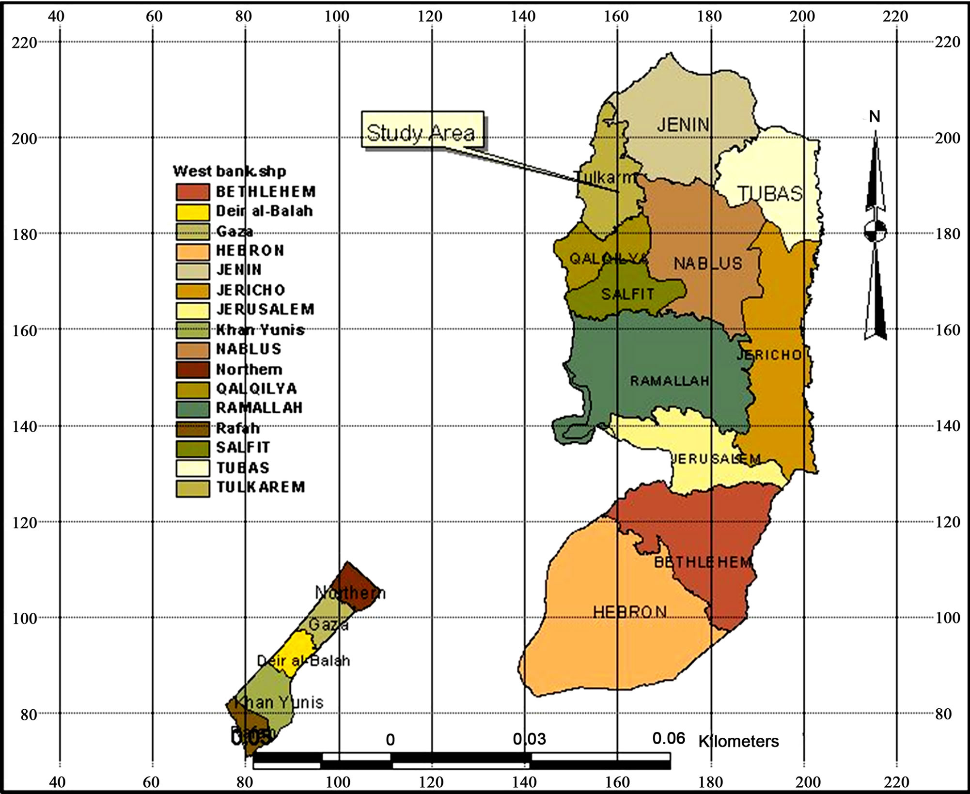
Figure 1. The location map of the study area.
3.2. Conceptual Model
The aim of the conceptual model is to define the requirements for the numerical model to be able to simulate water flow and with some restrictions transport phenomena for the region under steady state and transient conditions. The description of the model study area is shown in Figure 2.
The best representation of the aquifer system of the study area is described by a three-dimensional two layer models since the groundwater wells are located in the upper aquifer. The upper aquifer layer has a variable thickness ranging from 494 meters in the north western part of the model study area to 249 meters in different places. The second layer acts a confining layer (AquitardYatta formation) separating the upper and lower aquifer. The aquifer system is highly affected by geological faults and folded structures which make the possibility of a hydraulic connection between the different aquifers very high.
3.3. Boundary Conditions
The horizontal boundaries of the model domain are shown in Figure 3. The northern and southern boundaries of the study area are all of the no-flow boundary type.
The eastern boundary is of no flow boundary (water divide boundary). The western boundary is a specified head boundary of 24 m. The boundary conditions for the model were defined based on the static groundwater levels performed by SUSMAQ [7].
The model of the study area is located within the upper aquifer hydrogeology with (Hebron, Jerusalem, Bethlehem—named ) geological formation for over 77% of the model area. So, the aquifer properties were assumed to be the same for all the model study area ignoring the properties of other geological formations. A base map was constructed by the arcview GIS software, representing the model domain, its boundaries and wells locations. This map was exported as DXF-format (vector file) to be used by the Modflow software. The model boundary conditions were defined in the program and the surrounding cells were represented as inactive cells.
3.4. Aquifer Geometry and Aquifer Properties
Getting the accurate geometry of the aquifer system represented by the top and bottom of the model layers was the most difficult and challenging effort required to complete the model setup. The x, y, z coordinates for the upper aquifer and aquitard (Yatta Formation) layers were converted to (*.dat format) to be convenient with the

Figure 2. Description of the model study area.
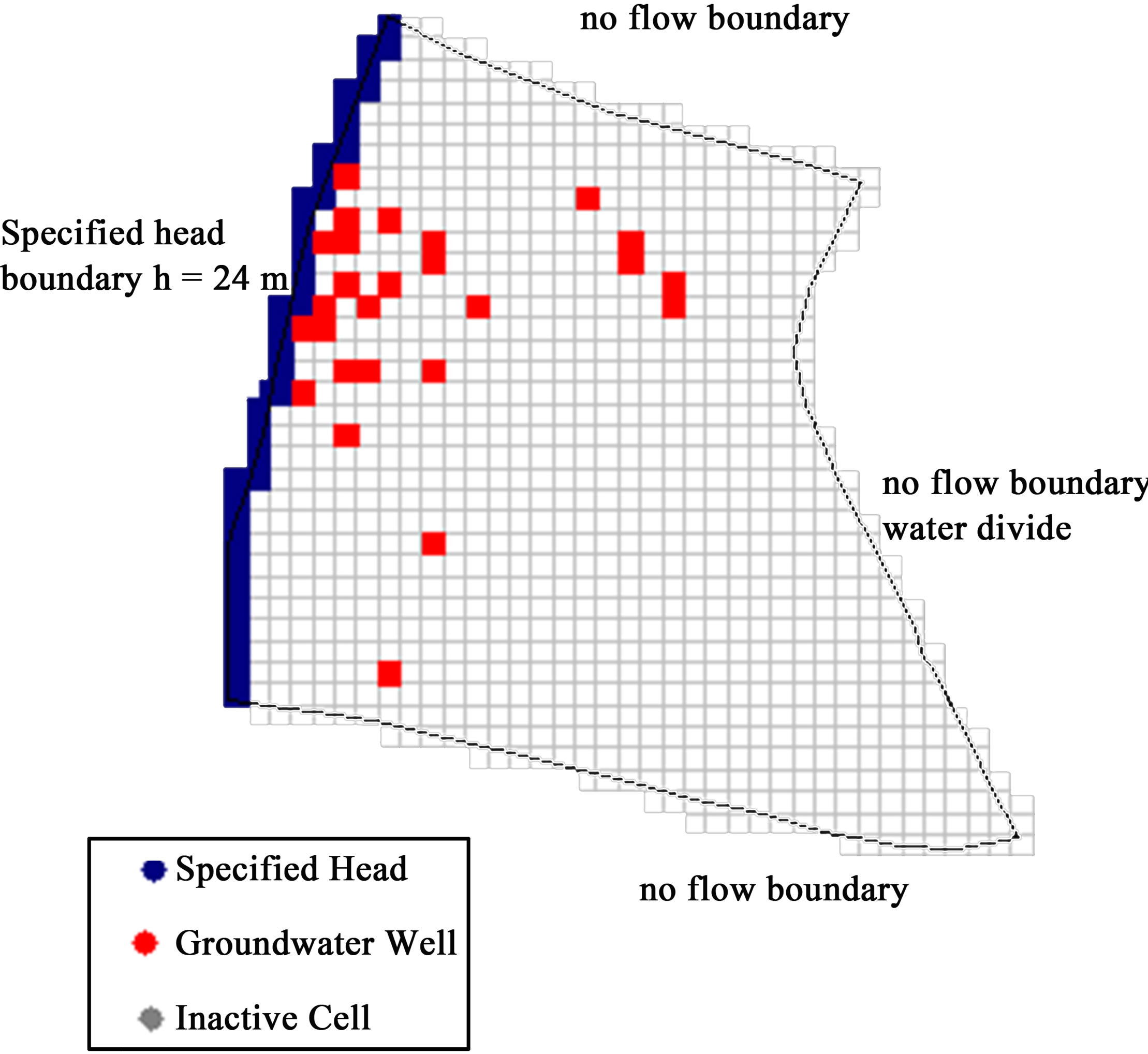
Figure 3. Model boundary conditions.
modflow software. In other words, this technique is mainly based on interpolating grids from coordinates using the field interpolator package under the Modflow software. There are no available hydraulic conductivity measurements for different aquifer layers of the WAB (Figure 4). The hydraulic conductivity of the fractured limestone and dolomite, which is characterizing the WAB area, is ranging from 1E–07 meters per second (0.00864 meters per day) to 6E–04 meters per second (51.84 meters per day) [9]. The Upper Aquifer is mainly composed of fractured limestone and dolomite which gave it relatively higher hydraulic conductivity. The Aquitard layer (Yatta Formation) is mainly composed of crystalline limestone and massive dolomite which gave it much lower hydraulic conductivity relative to upper layers. The average initial value of the horizontal hydraulic conductivity of the upper layer used in this model was 20 meters per day. The average initial value of the horizontal hydraulic conductivity of the aquitard layer used in this model was 0.1 meters per day and the vertical hydraulic conductivities assumed 1/10 of the horizontal conductivities for both layers. These values were based on the spatial distribution of the calibrated hydraulic conductivities done by SUSMAQ-[7].
3.5. Recharge Estimation & Wells Abstraction
Goldschmidt and Jacoub (1958) derived a relationship between recharge and runoff based on the long-term average rainfall over the catchment’s area. The empirical equation developed was based on the annual rainfall quantities during the period 1943\44 to 1953\54. The equation relates to the long term average total run off from a catchment (Rred) to the long term average precipitation over it (Pred).
Rred = 0.9 × (Pred – 360) in mm\yr
(Rred) in the above equation was approximated to equal the annual recharge R. This recharge value was divided into three segments to develop linear relationship between rainfall and recharge by Guttman and Zukerman [10]. The final equations developed could be read as follows:
R = 0.8 × (P – 360) P > 650 mm\yr
R = 0.534 × (P – 216) 650 > P > 300 mm\yr
R = 0.15 × (P) P < 300 mm\yr
R = Recharge from rainfall in mm\yr
P = Annual rainfall in mm\yr
The previous equations were applied to calculate the recharge for the model study area. Knowing that the average precipitation for the study area is to be (611.82 mm\yr), the estimated recharge is:
R = 0.534 (611.82 – 216)
= 211.37 mm\yr
= 0.00058 m\day
The pumpage of groundwater wells located within the model study area, was assumed to be (0.07 - 1) mcm\year for each well in the model study.
3.6. Model Simulation and Presentation
In order to run the model, values of hydraulic conductivities and recharge were assigned to each of the active cells
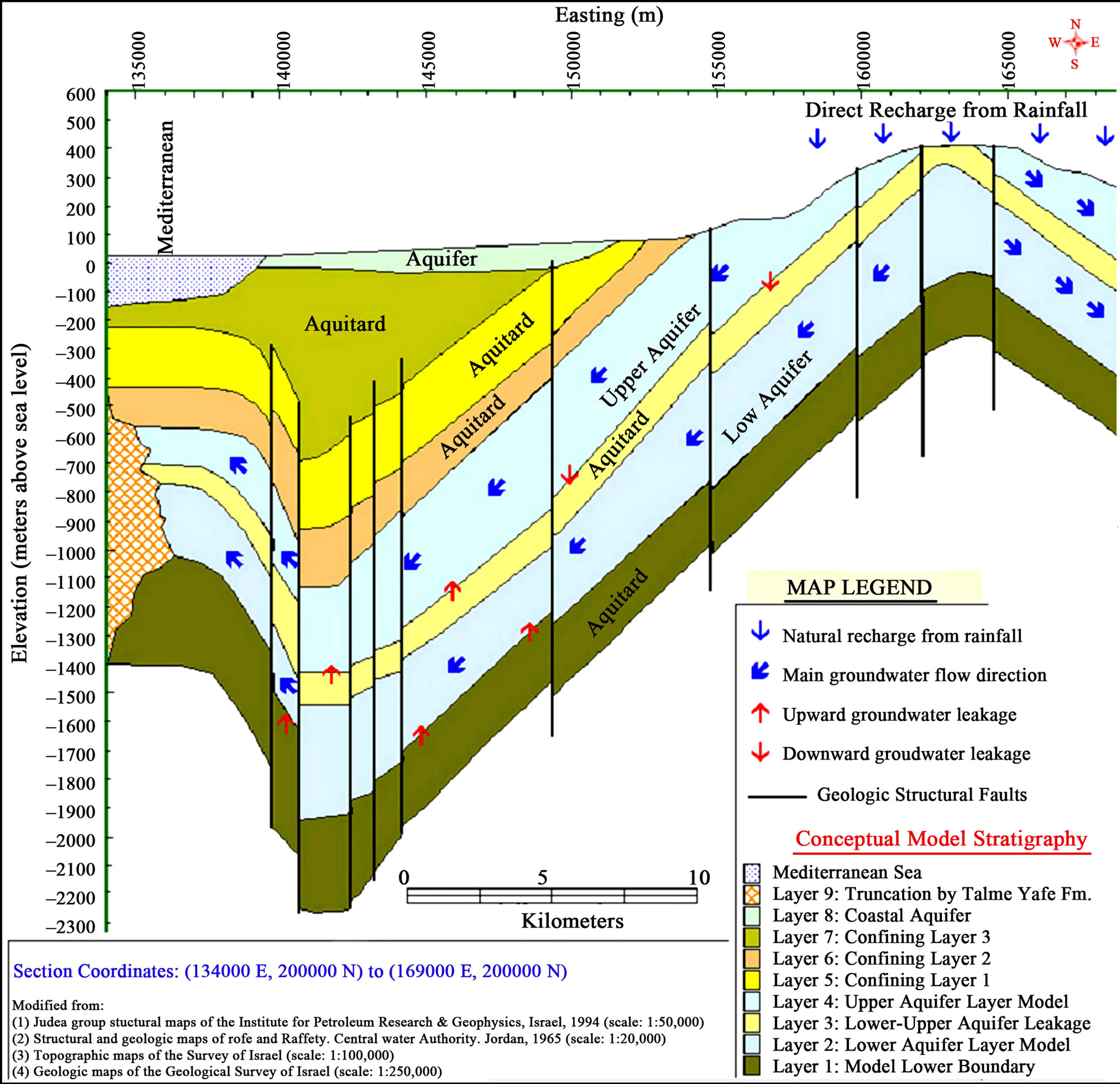 (Source: Sabbah, 2004)
Figure 4. East west hydro-geological cross section of WAB (northern area).
in the model domain. The result of the static groundwater level is shown in Figure 5. Several trials were conducted by assigning values of hydraulic conductivities spatially over the model domain and no change was observed through simulation. The results of the groundwater flow model can be listed as follows:
1) The groundwater head starts at an elevation of 110 meters above sea level (a.s.l.) in the south east of the area, 70 meters above sea level in the north east of the model and then it decreased gradually to a value of 24 meters above sea level in the western boundary of the model domain.
2) The model cells in the eastern part of the model area were dry which means that the computed head is lower than the bottom of the aquifer at these cells. That could be attributed to the fact that the model layers there are outcropped and to the absence of observation heads at that area. Also it may refer to the geometrical mistake within the model domain. In order to better account for that area with dry cells, the model could be updated by looking for more observations and by installing more pilot points of hydraulic conductivity there. The presence of dry cells may be justified by the recharge zone of the water divide boundary (no flow boundary).
3) Considering the simulated calculations of the aquifer system, the in-out flows from the groundwater reservoir can be defined as follows: The recharge to the aquifer in this model was calculated to be 25.15 MCM/year and the recharge through constant head was found to be 5.07 MCM/year. The discharge of groundwater wells was considered as outflow from the whole aquifer system and was calculated to be 21.5 MCM/year and the discharge through constant head was found to be 8.72 MCM/year. Table 1 shows the water flow budget of the whole model calculated on a yearly basis. inflow – outflow = 0.
The solute and transport model was simulated to investigate the movement of conservative pollutant using MT3D model. In this study a pollutant source of 2000 mg/L represented by built up areas (contaminated area) was used for model simulation (Figure 6). The input parameter affecting the movement of pollutant was also assumed to be 0.1 for effective porosity [7] and 50m for dispersivity, which is typical of karstic aquifer system. The response of pollution occurs due to dispersion and chloride concentration indicates a gradual increase with time up to high level after long term simulation for the model study area.
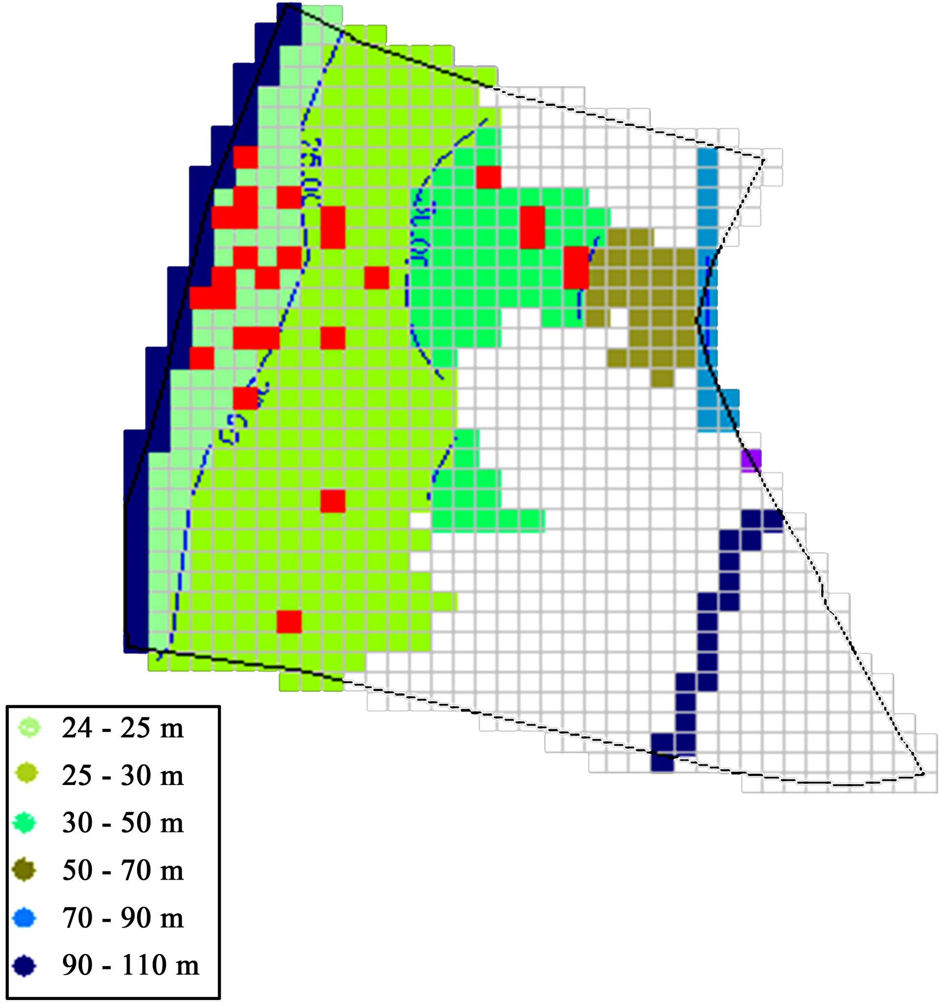
Figure 5. Static water level for the model domain.
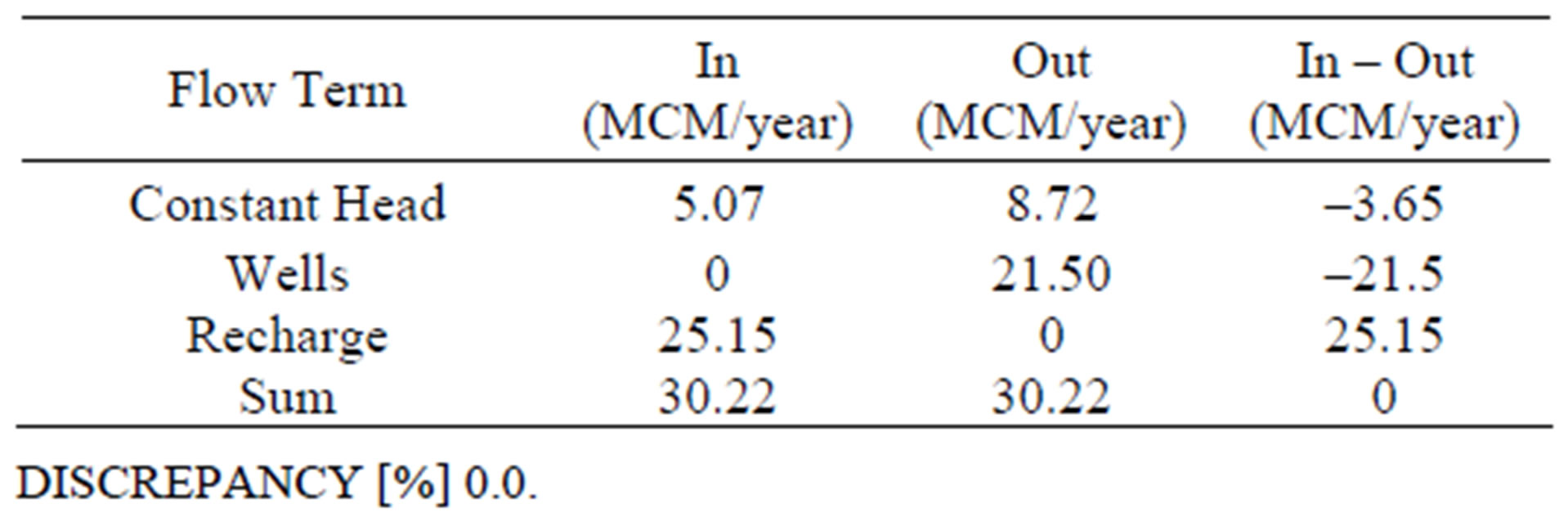
Table 1. Water flow budget of the whole model domain.

Figure 6. Chloride concentration at the end of simulation.
4. Conclusion
A 3-dimentional model of 2 layers system in the western portion of the north western part of Auja—Tamaseeh basin, which representing a high sensitive area of Tulkarm area was built using the Modflow software package. The groundwater head starts at an elevation of 110 meters a.s.l. in the south east of the area, 70 meters a.s.l. in the north east of the model, which indicates a flow direction to the north western parts. The in-out results of the model show of none percent discrepancy. The pollution model was built using the MT3D package under Modflow. The model output indicates that the response of pollution due to contaminant area chosen within the built-up areas shows that the tendency of contamination and pollutant spreading occurs due to dispersion. The results show that there is a gradual increase in chloride concentration with time during the period of simulation.
REFERENCES
- Palestinian Hydrology Group (PHG), “Hydrologicl Data Report,” Jerusalem, 2004.
- Palestinian Water Authority (PWA), “Master Data Bank,” Palestine, 2005.
- Ministry of Planning and International Cooperation— MOPIC, “Regional Plan for the West Bank Governorates: Water and Wastewater Existing Situation,” Palestine, 1998.
- Applied Research Institute in Jerusalem (ARIJ), “Environmental Profile for the West Bank: Tulkarm Area,” Palestine, 1996.
- Palestinian Central Bureau of Statistics (PCBS), “Area Statistics in the Palestinian Territories,” Ramallah, 2005.
- Rofe and Raffety Consulting Engineers, “West Bank Hydrology: Analysis Report (For the Central Water Authority of Jordan),” Westminister, London, 1965.
- SUSMAQ, “Steady State Flow Model for the Western Aquifer Basin,” Palestine, 2003.
- W. Sabbah, “Developing a GIS and Hydrological Modeling Approach for Sustainable Water Resources Management in the West Bank,” Palestine, 2004.
- P. Bedient, H. Rafai and C. Newell, “Groundwater Contamination,” Printice Hall, Upper Saddle Rive, 1999.
- Y. Guttman, and C. H. Zukerman, “A Model of the Flow in the Eastern Basin of the Mountains of Samaria from the Far’ah stream to the Jordan Desert,” Tahal, 1995.
NOTES
*Corresponding author.