Journal of Geographic Information System
Vol. 4 No. 2 (2012) , Article ID: 18786 , 8 pages DOI:10.4236/jgis.2012.42022
Conformal Analysis of Spatial Shift in High Resolution Satellite Data (HRSD)
1Department of Civil Engineering, Visvesvaraya National Institute of Technology, Nagpur, India
2ImaGIS Engineering Solutions Pvt. Ltd., Nagpur, India
Email: ybkatpatal@rediffmail.com, vasantmhaisalkar@yahoomail.com, *rohitms11@rediffmail.com
Received December 29, 2011; revised February 10, 2012; accepted February 22, 2012
Keywords: Spatial Shift; Ground Control Points; Rectification; Map Projection System; Transformation
ABSTRACT
Advent of High Resolution Satellite Data (HRSD) with development of high spatial resolution sensors have revolutionized the generation of large scale maps. Generation of large scale digital utility maps using HRSD involves different methodologies and includes several steps wherein errors or spatial shift may be induced at any stage of data generation. It may be interesting to note that the characteristics of the spatial shift vary with methodologies adopted in its processing and has unique implications with respect to the data usage along with its application. Spatial shifts of points on a satellite data is result of unexpected translation and rotation of pixel with respect to the original location. Present study analyzes the spatial shift generated in satellite data with reference to the change in area and orientation of a group of pixels i.e. conformal and equal area properties of the rectified satellite data. This study aims to establish a relationship between the spatial resolutions of the satellite image used for digital map generation with the spatial accuracy achieved. In this study, Ground Control Points (GCP’s) identified on satellite data for a sample study area were validated using Differential Global Positioning System. Five different high resolution satellite images were analyzed to verify changes in area and shape with reference to the GCP’s. The results indicate that with improvement in the spatial resolution, higher precision in the digital maps is accomplished in terms of spatial shift of the points.
1. Introduction
Resources management; especially the resources related to earth’s surface necessitate spatial database. Remotely sensed data gathered by satellite or aircraft are depictions of the irregular and curved surface of Earth. The spatial data are the numerical values, which represent the location, size and shape of objects found in the physical world [1]. Satellite remote sensing data is an important source of spatial data in today’s digital environment. But in raw format it contains geometrical misrepresentations, which make them unusable as geographically standard datasets [2]. In order to update and compile maps with high accuracy, it is vital to relate the satellite remote sensing data to a ground coordinate system [3].
Digital Mapping Techniques have been applied for generation and apprising the urban information [4]. Attempts have been made to study the errors generated in specific satellite data and specific processes involved in the digital data generation [5,6], But generally, it has been observed that accuracy of spatial data obtained through sensing remains a challenging area. Greenfeld [7] observed that major stumbling block to the effective application of spatial digital data is the positional accuracy of the spatial database. Exactitude of the satellite data can be increased by proper use of rectification techniques. But, the focus of the study here is to analyze and evaluate the variation in the accuracy achieved with increasing spatial resolution of different sensors, keeping the projection system and rectification techniques constant. This comparison has been presented here individually for three projection systems viz. Lambert Conformal Conic system with Everest 1956 datum (LCC/EVE1956), Polyconic projection system with Everest 1956 datum (PC/EVE 1956) and Universal Transverse Mercator projection system with WGS 84 datum (UTM/WGS84), each with first and second order of polynomial transformation technique.
2. Methodology
In this present study, a sample area was selected in northwest portion of Nagpur City, of Maharashtra State, located in Central-India. Satellite data with varying spatial resolution from 0.63 m to 30 m viz. Quickbird, IKONOS, Indian Remote Sensing (IRS) PAN, LISS III and Landsat TM were been used in this analysis for the sample study area. Indian satellite data from sensors like IRS-1D, LISS-III MSS and PAN merged products are widely used in urban analysis and urban land use mapping [8]. Seven Ground Control Points (GCP’s) were identified on the all the five (05) satellite data for which corresponding points on the ground were located. These were marked with nail on the site. The data was projected and rectified using the standard methods of geo-referencing. The datasets were transformed using three commonly used combinations of map projection system and datum in India viz. Lambert Conformal Conic system with Everest 1956 datum (LCC/ EVE1956), Polyconic projection system with Everest 1956 datum (PC/EVE 1956) and Universal Transverse Mercator projection system with WGS 84 datum (UTM/ WGS84). Polynomial transformation technique with first and second order of transformation was used to transform the datasets.
The sample area was surveyed using Differential Global Positioning System (DGPS) and a basemap was prepared in UTM map projection system and WGS84 datum. The basemap was cross checked by a detailed Total station traverse using TRIMBLE make 3602DR total station theodolite, to collect the coordinates of the seven GCP’s. Proper closing of the traverse was done as per standard procedures and the closing error was distributed evenly using the Bowditch rule in all the traverse stations [9]. The variation in the lengths observed using the DGPS and Total station technique was 0.027 m in 1 km, which was tolerable for the large scale urban mapping applications. By this technique, exact orthographic distance between the control points was calculated. The basemap was used as reference for computing the spatial shift in various satellite data. The spatial shift in the data was used to compute the variation in the area enclosed by a group of pixels after rectification of the data.
3. Analysis
The spatial shift of the data was a result of two processes;
• Translation;
• Rotation.
Translation is the shift of points in a straight line while rotation indicates angular shift of the points with respect to its original location.
Spatial shift = shift due + shift to translation due to rotation
The spatial shift in the satellite data due to translation and rotation is analyzed by computing and studying the change in size and shape of an area covered by a group of pixels and studying the movement of GCP’s before and after its rectification. The study has been divided in two aspects viz. Equal area analyses and Orientation analyses. Equal area analysis was carried out by comparing the variation in size of an area covered by a group of pixels in the rectified satellite data and the area covered by the same group of pixels in reference basemap. This analysis is termed as the “Equal Area analysis”.
For conformality analysis, one centroid was mathematically located and the bearing/direction of the line joining the GCP’s and centroid of the triangulated area was measured. Then the rotation of the GCP’s with respect to the centroid of the area was computed. The centroid of the area of the group of pixels was computed mathematically for all the data sets. This analysis of the conformality property of the map projection was termed as the “Orientation analysis”.
3.1 Equal Area Analysis
The spatial shift in the data ultimately results in error in the area and shape of area of interest. To study this conformal behavior, the study of shift was carried out by analyzing the change in area enclosed by the GCP’s. The area analysis was carried out using the standard formulae for computing the area and perimeter of the triangle.
Equal area analysis was carried out for the area enclosed within the seven (07) GCP’s in five (05) triangles, termed as Area of Interest (AOI) as shown in the Figure 1. The area of each triangle was computed for satellite data from all the sensors and combinations of map projection system and order of transformation. The perimeter of the triangles was also computed and checked to assess the linear variation in the perimeter of the triangular areas. The area of triangles of the reference basemap prepared from the DGPS data in UTM/WGS-84 projection system was taken as reference for the comparative analysis. Total area of the five (05) triangles was 465 Hectare in the reference basemap.
The change in total area, quantified as the percentage change in area, for data from various sensors was compared with the area computed from the reference DGPS data. The Percentage (%) variation in area/Hectare for all the data sets is calculated indicating the usability of the data for the applications involving area computation studies.
3.2 Orientation Analysis
The Orientation analysis studies the clockwise or anticlockwise rotation of the pixel from the input location after rectification. To analyze the rotation aspect, the centroid of the AOI was calculated for each data sets and the initial and final location of the pixel was analyzed with respect to the centroid of the AOI. The formulae used for the computation of the coordinates of centroid and the rotation angle are listed below. Katpatal and Mane [10] have studied the change in orientation of coordinates in linear corridors and have presented methodology to minimize it through selection of suitable projection parameters. Figure 2 shows the AOI enclosed by GCP’s and the centroid of the AOI. The input and the transformed location of the GCP’s are plotted and the
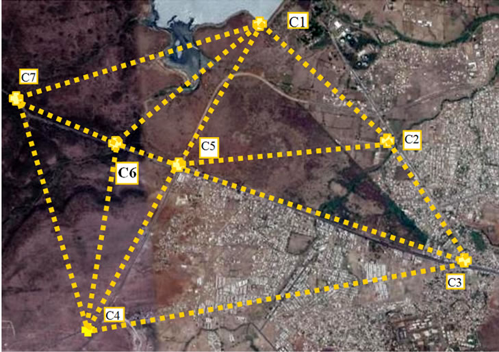
Figure 1. Area of interest with five triangles used for area computation study.

Figure 2. AOI enclosed by GCP’s and centroid.
distance and bearing of each GCP is measured with respect to the centroid of the AOI. The North-bearing of line joining the centroid and the GCP with respect to the north direction gives clockwise or anticlockwise rotation of the GCP after rectification. The distance of the pixel from centroid also changes resulting in the non-uniform change in the data.
The formulae for computing centroid of triangles
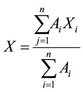
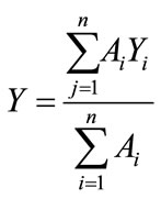
where A = area of each triangle;
xi = x coordinate of centroid of each triangle;
yi = y coordinate of centroid of each triangle;
i = no. of triangles;
X = x coordinate of centroid of all triangles;
Y = y coordinate of centroid of all triangles;
Rotation angle with respect to centroid = θ – θ'.
where
θ = Bearing of input GCP;
θ' = Bearing of transferred GCP.
Distance from origin = 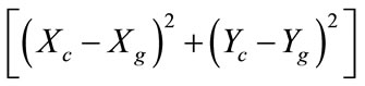
where Xc = X coordinate of centroid;
Yc = Y coordinate of centroid;
Xg = X coordinate of GCP;
Yg = Y coordinate of GCP.
4. Results
4.1. Equal Area Analysis
The area enclosed by the five (05) triangles (AOI) was computed mathematically for all the combinations of satellite data and projection systems and was checked with the area of the triangles of the DGPS reference base map. The perimeter of the triangles was also checked for variation in the perimeter compared to the reference basemap. Table 1 shows the variation in total area and perimeter of AOI for Quickbird data for the various combinations of map projection system and order of transformation.
As evident in Figure 3, Quickbird data shows minimum variation of area of five (05) triangles and perimeter for UTM/WGS-84 map projections system with first order of transformation. The minimum area variation is 0.102%, i.e. 10.20 sqm/ha in case of 1st Order UTM/ Wgs84 which is very less and acceptable for large scale mapping.
Table 2 shows the variation in total area and perimeter of AOI for Ikonos data for the various combinations of map projection system and order of transformation.
The result shows that the variation in area was least in case of Ikonos UTM/WGS-84 data with second order transformation (Figure 4). The spatial shift was minimum for same combination of data and hence the variation in area was also minimum. The variation is 319 sqm in total area of 4,651,646 sqm, which is just 0.007% or it can be represented as a variation of 0.7 sqm in one Hectare. Similarly; area variations of IRS PAN, LISS III and Landsat data were computed. Table 3 shows abstract of the variation in area of triangles for various combinations of projection system and order of transformation.
The variation is represented in percentage, which is least in case of UTM/WGS-84 projection system in Ikonos
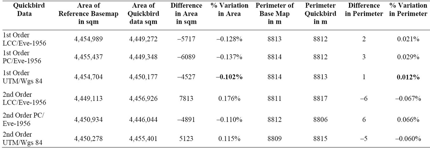
Table 1. Comparison of the variation in area and perimeter for Quickbird data and reference Basemap.
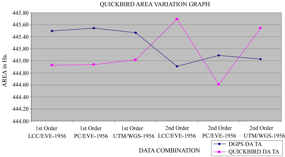
Figure 3. Variation in area of Quickbird data for various combinations of map projection systems.

Table 2. Comparison of the variation in area and perimeter for Ikonos data and absolute Basemap.
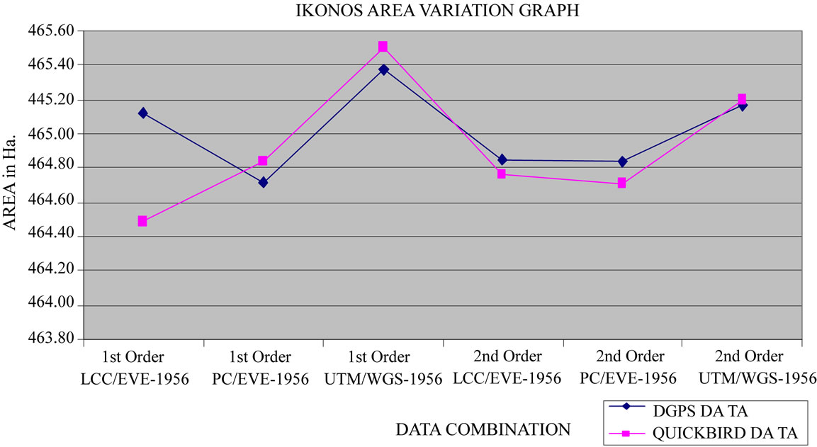
Figure 4. Variation in area of AOI for Ikonos data for various combinations of map projection systems.
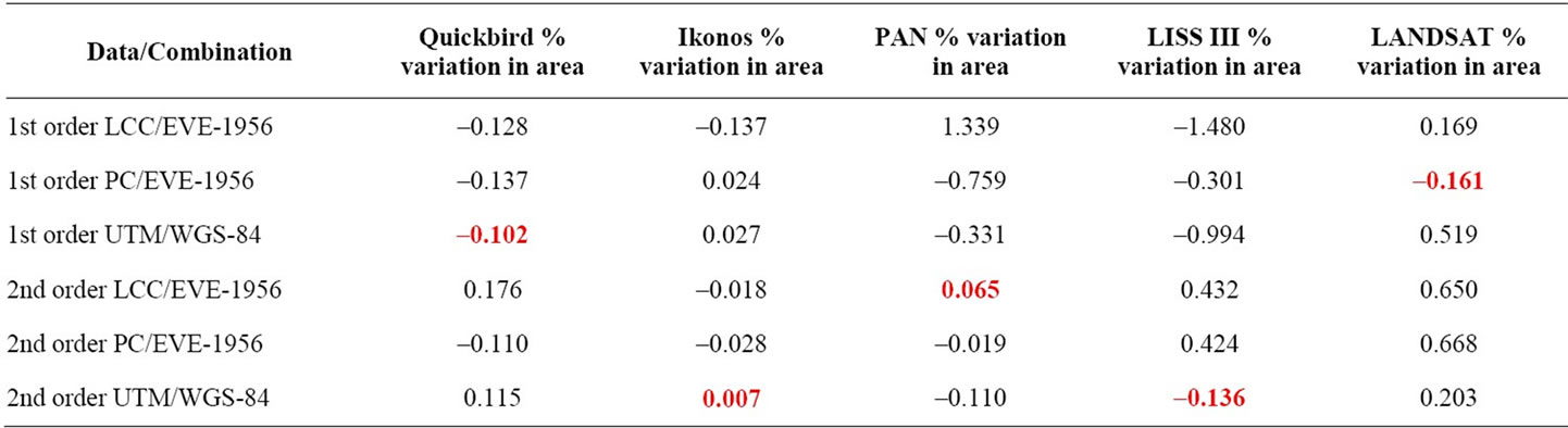
Table 3. Abstract of the percentage variation in area of triangles for five data sets.
data for the second order transformation and PC/EVE- 1956 projection system. The percentage (%) variation in area is converted to equivalent variation in sqm per hectare (sqm/ha) area as shown in Table 4.
Figure 5 shows that for Ikonos and PAN data, the variation in the area ranges between 1 - 2 sqm/ha, which is permissible. This can be effectively used to generate the large scale thematic maps. But Quickbird and all other datasets show more than 10 sqm/ha area variations. In case of other datasets, the variation increases and achieving even this much accuracy is difficult for larger areas, hence it should be used prudently for generation of thematic maps.
4.2 Orientation Analysis of the Data
The spatial shift in the data is explained as the shift of a point or pixel to a new location. Table 5 shows the rotation of the GCP’s for first order transformation of Ikonos UTM/WGS-84 data compared with DGPS reference basemap for first order transformation.
The rotation of the GCP’s has been plotted as “Polar plots” showing the initial and transformed location of each pixel with respect to the centroid. Polar plots display GCP’s in the coordinate system format. Herein the distance from the origin or centroid of the graph, and theta (θ) are the angle between the positive horizontal axis and the radius vector extending from the centroid to the GCP. The radius of the Polar plot is taken as the distance from the centroid of the AOI and the GCP’s; which are plotted using the north-bearing of the line from the centroid and the distance from centroid. Figure 6
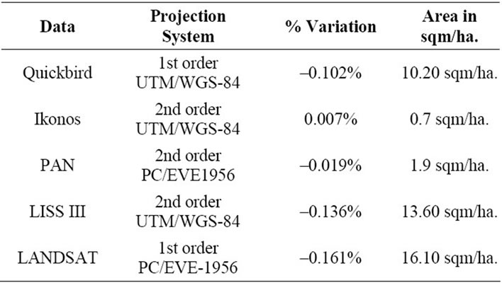
Table 4. Variation in area represented in sqm/ha.
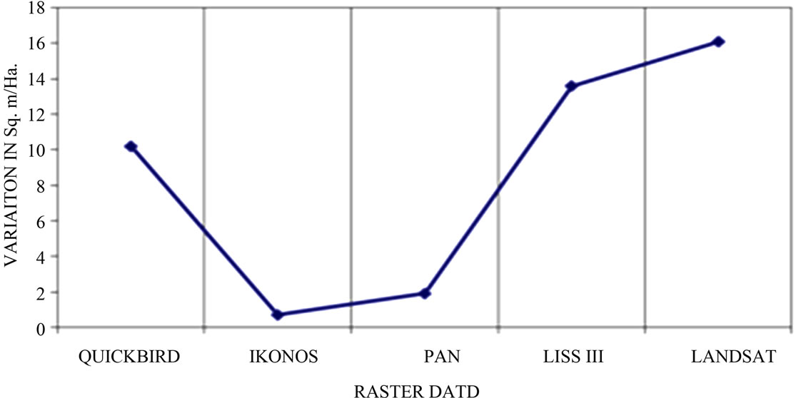
Figure 5. Area variation in sqm/ha for various data sets.
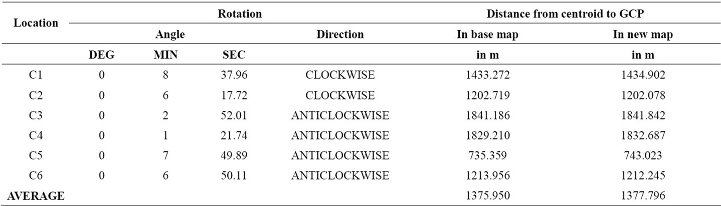
Table 5. Rotation of the GCP’s for first order transformation of Ikonos UTM/WGS-84 data compared with DGPS basemap for first order transformation.
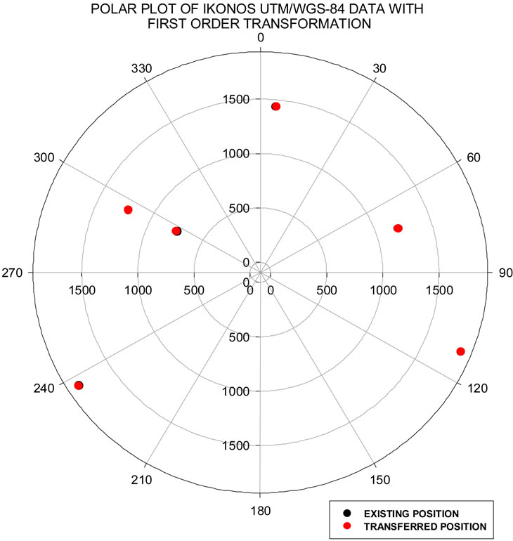
Figure 6. Polar plot of Ikonos UTM/WGS-84 data with first order transformation.
shows the polar plot for Ikonos UTM/WGS-84 data for first order transformation. The Polar plots of LISS III LCC/EVE-1956 data and Landsat UTM/WGS-84 data with first order transformation is shown in Figures 7 and 8 respectively.
The rotation at the GCP’s is averaged to compute the rotation of the AOI in the image. The spatial shift in the satellite data is the result of the transformation of the GCP’s and is represented in the form of rotation of the pixels. The rotation at the GCP locations for Ikonos data for six (06) combinations of projection system is illustrated in the Figure 9. The graph shows that the rotation was least in respect for GCP No. C2, C3 and C4.
They were extreme (very high) for GCP No. C5 for PC/ EVE-1956 projection system with second order transformation.
This average rotation for various combinations of transformation is represented graphically in Figure 10 for various datasets. It is obvious form the graph (Figure 10) that second order transformation results in less rotational shift compared to the first order transformation. The improvement is substantial in case of the low resolution satellite images compared to high resolution images. Table 6

Figure 7. Polar plot of LISS III LCC/EVE-1956 data with first order transformation.
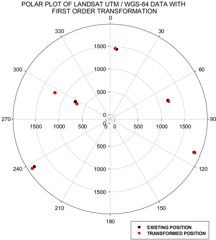
Figure 8. Polar plot of Landsat UTM/WGS-84 data with first order transformation.
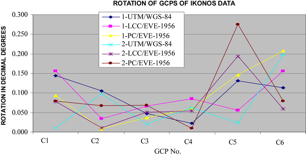
Figure 9. Rotation at the GCP’s for Ikonos data for various combinations of projection systems.
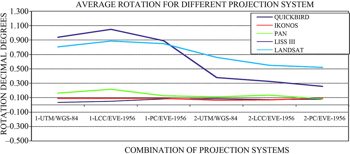
Figure 10. Average rotation for different projection system for various data sets.
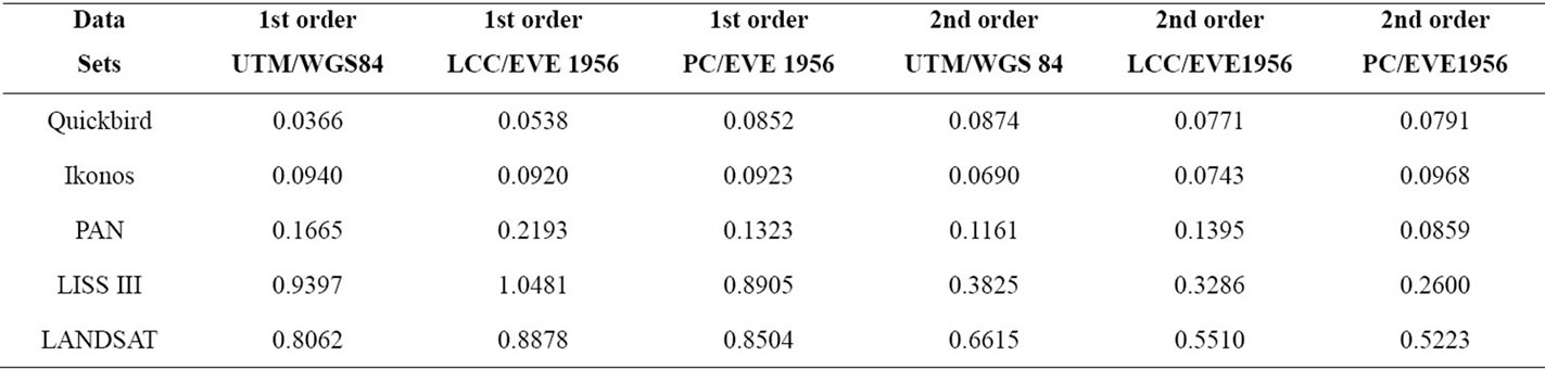
Table 6. Average rotation in decimal degrees for different datasets for different combinations of map projection system and order of transformation.
shows average rotation of the GCP’s for various datasets for six combinations of map projection system and order of transformation. The rotation for Quickbird, Ikonos and PAN data is minimum followed by Landsat and LISS III data. Overall, the second order transformation shows less rotation i.e. less shift compared to the first order transformation.
5. Conclusions
This study emphatically establishes for the fact that; Spatial Resolution of satellite data and conformal properties of map projections affect the dimensional accuracy of the digital data generated, totally based on the following conclusions. This are totally drawn based on the study as elucidated below:
● It has been observed that percentage variation are least in case of UTM/WGS-84 projection system of Ikonos data for the second order transformation and second order PC/EVE-1956 projection system (Ref Table 4).
● The variation in area in sqm/ha for Ikonos and PAN data ranges between 1 - 2 sqm/ha, which are permissible.
● This can be effectively used to generate the large scale thematic maps. But, for Quickbird and all other datasets the variation is somewhat more.
● The rotation of the coordinates for Quickbird, Ikonos and PAN data was minimum followed by Landsat and LISS III data.
● Overall, the second order transformation show less rotation i.e. small angular shift as compared to the first order transformation.
OPINE:
● High resolution satellite data is being used nowadays for many large scale urban mapping applications.
● There is growing tendency to use satellite data with spatial resolution as high as 0.50 m.
● The present study attempted to analyze conformaly the spatial shift in a data with reference to the change in area and orientation of the pixels due to change in map projection system and order of transformation of the data.
● The results showed that the effect of spatial shift in the data is reduced considerably in case of satellite data with high spatial resolution.
● The study also indicates that higher spatial resolution satellite data may be utilized for large scale digital mapping projects for various applications.
REFERENCES
- E. F. Burkholder, “Spatial Data Coordinate Systems and the Science of Measurement,” Journal of Surveying Engineering, Vol. 127, No. 4, 2001, pp. 143-156. doi:10.1061/(ASCE)0733-9453(2001)127:4(143)
- V. K. Srivastav, “Significance of Global Positioning System (GPS) Measurements in Geo-Referencing of Remote Sensing Images an Input in GIS,” Proceedings of the Asian GPS Conference, New Delhi, 29-30 October 2001.
- P. Nag and M. Kudrat, “Digital Remote Sensing,” Concept Publishing Company, New Delhi, 1998.
- R. S. Rathi and R. R. Vatsvani, “Digital Mapping of Urban/Sub-Urban Environment of Dehradun Using SPOT Data,” In: B. S. Sokhi and S. M. Rashid, Eds., Remote Sensing of Urban Environment, Manak Publications, New Delhi, 1999, pp. 123-136.
- H. Hild, “Automatic Image-to-Map-Registration of Remote Sensing Data,” Photogrammetric Week, 13-23 January 2001.
- A. Shaker, W. Shi and H. Bharakat, “Assessment of the Rectification Accuracy of Ikonos Imagery Based on TwoDimensional Models,” International Journal of Remote Sensing, Vol. 26, No. 4, 2005, pp. 719-731. doi:10.1080/01431160512331316847
- J. Greenfeld, “Evaluating the Accuracy of Digital Orthophoto Quadrangles (DOQ) in the Context of Parcel-Based GIS,” Photogrammetric Engineering and Remote Sensing, Vol. 67, No. 2, 2001, pp. 199-205.
- Indian Space Research Organisation, “Urban Planning Using IRS-1C Data,” ISRO, Bangalore, 2005.
- A. Bannister, R. Stanley and R. Baker, “Surveying,” Pearson Education, India, 2006.
- Y. B. Katpatal and R. S. Mane, “Minimizing the Edge Distortions in Spatial Representation of Standard UTM Zones Using GPS: A Case Study,” Proceedings of the International Conference on Location Intelligence, New Delhi, 2-4 May 2005.
NOTES
*Corresponding author.