Journal of Modern Physics
Vol.5 No.6(2014), Article ID:45321,5 pages DOI:10.4236/jmp.2014.56052
Pair Production in Non-Perturbative QCD
Salah Hamieh
Department of Physics, Faculty of Sciences, Lebanese University, Beirut, Lebanon
Email: hamiehs@yahoo.fr
Copyright © 2014 by author and Scientific Research Publishing Inc.
This work is licensed under the Creative Commons Attribution International License (CC BY).
http://creativecommons.org/licenses/by/4.0/


Received 8 January 2014; revised 5 February 2014; accepted 3 March 2014
ABSTRACT
In this paper, a method to calculate the vacuum to vacuum transition amplitude in the presence of a non-abelian background field is introduced. The number of non-perturbative quark-antiquark produced per unit time, per unit volume and per unit transverse momentum from a given constant chromo-electric field is calculated and its application to quark-gluon plasma is presented.
Keywords:Pair Production, Non-Perturbative QCD

1. Introduction
Lattice QCD predicts a phase transition from Hadrons gaz (HG) to quark-gluon plasma (QGP) at deconfinement temperature, T  170 MeV. It is believed that QGP has been produced in relativistic heavy ions collision [1] -[4] where in the initial pre-equilibrium stage of QGP about half the total center-of-mass energy,
  , goes into the production of a semi-classical gluon field [5] -[17] . Therefeore, to study the production of a QGP from a classical chromo field, it is necessary to know how quarks and gluons are formed from the latter. The production rate of quark-antiquark from a given constant chromo-electric field
  has been derived in Ref. [18] and the integrated
  distribution has been obtained in [19] -[22] (for a review see [23] ).
In this short technical note, we will extend the results of Ref. [18] to a general constant background field. The method presented here may simplify the complexity found in the Non-perturbative QCD calculations. Also, the obtained  distribution for quark (antiquark) production can be used in the analysis of the experimental results at the RHIC and the LHC colliders.
The paper is organized as follows: in the next section, we will calculate the one loop effective action needed in the evaluation of the  distribution of the quark (antiquark) production. In Section 3 the
  distribution is presented. Finally, in Section 4, an application to heavy ion collision is given.
2. The One Loop Effective Action
As described in the above section, we will evaluate here the one loop effective action in the presence of a constant chromo-field. For this purpose, we start from the QCD Lagrangian density for a quark in a non-abelian background field  which is given by
 (1)
(1)
Then the vacuum to vacuum transition amplitude is given by
 (2)
(2)
And the one loop effective action can be written in this form
 (3)
(3)
Thus, using the invariance of trace under transposition and the following relation
 (4)
(4)
we obtain the following expression1
 (5)
(5)
The quickest way to calculate the effective action is to work in a basis  that are the eigenstates of
  defined by:
 (6)
(6)
which is a part of the one loop effective action ![]() of Equation (5).
of Equation (5).
As an application to this idea, we first consider the case of a constant electric field in the  direction (direction of the beam in the heavy ion collision). In this case, we choose a gauge such that we can take
 . Thus the second part of Equation (6) can be written in this form
 (7)
(7)
The Hamiltonian becomes
 (8)
(8)
After a straightforward algebra one can find the following eigenvalues of the Hamiltonian 
 (9)
(9)
where  are the eigenvalues over the Dirac matrices such that
  and
and . And
. And![]() , with
, with , are the eigenvalue for
  over the group space and are given by [18] .
 (10)
(10)
with ![]() given by
given by
 (11)
(11)
where
 (12)
(12)
Using the obtained eigenvalues of the Hamiltonian , the effective action becomes
 (13)
(13)
Performing the i and n summations we found
 (14)
(14)
which is the same results as Ref. [18] . Clearly, the one loop magnetic effective action can be found upon the following substitution . Therefore
 (15)
(15)
3. Pair Production in Non-Perturbative QCD
Now, in the same manner as in Ref. [18] we may derive the non-perturbative quarks (antiquarks) production per unit time, per unit volume and per unit transverse momentum from a given constant chromo-electric field . Thus as done in Ref. [18] we can find that
 (16)
(16)
where  is the effective mass of the quark and the eigenvalues
 ![]() are given above.
are given above.
4. Application to Heavy Ion Collisions
Let's consider the situation of two relativistic heavy nuclei colliding and leaving behind a semi-classical gluon field which then non-perturbatively produces gluon and quark-antiquark pairs via the Schwinger mechanism [19] . As estimated in Ref. [24] for Au-Au collision at RHIC collider with ![]() fm and center-of-mass energy
fm and center-of-mass energy ![]() GeV per nucleon, the initial energy density is
GeV per nucleon, the initial energy density is  GeV4 and
  GeV4. For our analysis we take
 ![]() which can be justified by the sensitivity check that has been made in Ref. [24] where it has been found that the production rate is not very sensitive to
which can be justified by the sensitivity check that has been made in Ref. [24] where it has been found that the production rate is not very sensitive to .
.
In Figure 1 we plot the rate of quark production as a function of the transverse momentum for two values of  (used in [25] ) and
  with initial energy density
  GeV4. Clearly seen from this figure that the production rate decrease with
  and becomes negligible at
  GeV. The obtained
  distribution for quark (antiquark) production can be used to fix the initial conditions for the QGP in heavy ion collision at the RHIC and the LHC colliders.
5. Conclusion
In this note we have proposed a method for calculating the vacuum to vacuum transition amplitude in the presence of the non-abelian background field. The method can be applied to a general background field and it can be updated to study the non-perturbative soft gluon production [26] . Also, we have evaluated the rate for
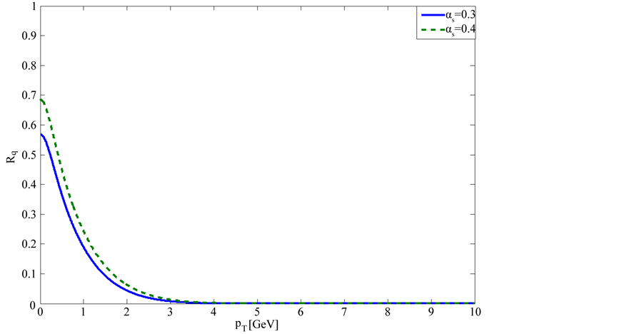
Figure 1. (Color online) Transverse production rate for quarks for  for
for , as a function of
 . For simplicity we denote here the quark production rate given in Equation (16) by
![]() . We take
. We take![]() ,
,  GeV.
GeV.
quark (antiquark) production in a constant chromo-electric field . These results are used to determine the quark (antiquark) production rate in heavy ion collision.
References
- Collins, J.C. and Perry, M.J. (1975) Physical Review Letters, 34, 1353. http://dx.doi.org/10.1103/PhysRevLett.34.1353
- Karsch, F., Laermann, E. and Peikert, A. (2000) Physics Letters B, 478, 447-455. http://dx.doi.org/10.1016/S0370-2693(00)00292-6
- Hamieh, S., Letessier, J. and Rafelski, J. (2003) Physical Review A, 67, Article ID: 014301. http://dx.doi.org/10.1103/PhysRevA.67.014301
- Hamieh, S., Redlich, K. and Tounsi, A. (2004) Journal of Physics G, 30, 481, http://dx.doi.org/10.1088/0954-3899/30/4/007
- Baym, G. (1984) Physics Letters B, 138, 18-22. http://dx.doi.org/10.1016/0370-2693(84)91863-X
- Kajantie, K. and Matsui, T. (1985) Physics Letters B, 164, 373-378. http://dx.doi.org/10.1016/0370-2693(85)90343-0
- Eskola, K.J. and Gyulassy, M. (1993) Physical Review C, 47, 2329. http://dx.doi.org/10.1103/PhysRevC.47.2329
- Nayak, G.C. and Ravishankar, V. (1997) Physical Review D, 55, 6877. http://dx.doi.org/10.1103/PhysRevD.55.6877
- Nayak, G.C. and Ravishankar, V. (1998) Physical Review C, 58, 356. http://dx.doi.org/10.1103/PhysRevC.58.356
- Bhalerao, R.S. and Nayak, G.C. (2000) Physical Review C, 61, Article ID: 054907. http://dx.doi.org/10.1103/PhysRevC.61.054907
- Kluger, Y., Eisenberg, J.M., Svetitsky, B., Cooper, F. and Mottola, E. (1991) Physical Review Letters, 67, 2427; http://dx.doi.org/10.1103/PhysRevLett.67.2427
- Kluger, Y., Eisenberg, J.M., Svetitsky, B., Cooper, F. and Mottola, E. (1992) Physical Review D, 45, 4659. http://dx.doi.org/10.1103/PhysRevD.45.4659
- Kharzeev, D. and Tuchin, K. hep-ph/0501234.
- McLerran, L. and Venugopalan, R. (1994) Physical Review D, 50, 2225. http://dx.doi.org/10.1103/PhysRevD.50.2225
- Dietrich, D.D., Nayak, G.C. and Greiner, W. (2001) Physical Review D, 64, Article ID: 074006. http://dx.doi.org/10.1103/PhysRevD.64.074006
- Gyulassy, M. and McLerran, L. (1997) Physical Review C, 56, 2219. http://dx.doi.org/10.1103/PhysRevC.56.2219
- Dietrich, D.D. Physical Review D, 7.
- Nayak, G.C. and Van Nieuwenhuizen, P. (2005) Physical Review D, 72, 125010. http://dx.doi.org/10.1103/PhysRevD.72.125010
- Schwinger, J. (1951) Physical Review, 82, 664. http://dx.doi.org/10.1103/PhysRev.82.664
- Claudson, M., Yildiz, A. and Cox, P.H. (1980) Physical Review D, 22, 2022. http://dx.doi.org/10.1103/PhysRevD.22.2022
- Casher, A., Neuberger, H. and Nussinov, S. (1979) Physical Review D, 20, 179. http://dx.doi.org/10.1103/PhysRevD.20.179
- Glendenning, N.K. and Matsui, T. (1983) Physical Review D, 28, 2890. http://dx.doi.org/10.1103/PhysRevD.28.2890
- Dunne, G.V. (2004) Heisenberg-Euler Effective Lagrangians: Basics and Extensions, hep-th/0406216. In: Shifman, M., et al., Eds., From Fields to Strings, Vol. 1, 445-522.
- Cooper, F., Dawson, J.F. and Mihaila, B. (2008) Physical Review D, 78, 117901. http://dx.doi.org/10.1103/PhysRevD.78.117901
- Aurenche, P. and Zakharov, B.G. arXiv:1205.6462 [hep-ph].
NOTES

1see Ref. and reference therein.