Applied Mathematics
Vol.06 No.14(2015), Article ID:62500,14 pages
10.4236/am.2015.614206
The Odd Generalized Exponential Gompertz Distribution
M. A. El-Damcese1, Abdelfattah Mustafa2, B. S. El-Desouky2, M. E. Mustafa2
1Department of Mathematics, Faculty of Science, Tanta University, Egypt
2Department of Mathematics, Faculty of Science, Mansoura University, Egypt

Copyright © 2015 by authors and Scientific Research Publishing Inc.
This work is licensed under the Creative Commons Attribution International License (CC BY).
http://creativecommons.org/licenses/by/4.0/


Received 6 November 2015; accepted 28 December 2015; published 31 December 2015
ABSTRACT
In this paper we propose a new lifetime model, called the odd generalized exponential gompertz distribution. We obtained some of its mathematical properties. Some structural properties of the new distribution are studied. The method of maximum likelihood is used for estimating the model parameters and the observed Fisher’s information matrix is derived. We illustrate the usefulness of the proposed model by applications to real data.
Keywords:
Gompertz Distribution, Hazard Function, Moments, Maximum Likelihood Estimation, Odds Function, T-X Family of Distributions

1. Introduction
In the analysis of lifetime data we can use the Gompertz, exponential and generalized exponential distributions. It is known that the exponential distribution has only constant hazard rate function where as Gompertz and generalized exponential distributions can have only monotone (increasing in case of Gompertz and increasing or decreasing in case of generalized exponential distribution) hazard rate. These distributions are used for modelling the lifetimes of components of physical systems and the organisms of biological populations. The Gompertz distribution has received considerable attention from demographers and actuaries. Pollard and Valkovics [1] were the first to study the Gompertz distribution, they both defined the moment generating function of the Gompertz distribution in terms of the incomplete or complete gamma function and their results are either approximate or left in an integral form. Later, Marshall and Olkin [2] described the negative Gompertz distribution; a Gompertz distribution with a negative rate of aging parameter.
Recently, a generalization of the Gompertz distribution based on the idea given in [3] was proposed by [4] this new distribution is known as generalized Gompertz (GG) distribution which includes the exponential (E), generalized exponential (GE) and Gompertz (G) distributions. A new generalization of th Gompertz (G) distribution which results of the application of the Gompertz distribution to the Beta generator proposed by [5] , called the Beta-Gompertz (BG) distribution which introduced by [6] . On the other hand the two-parameter exponentiated exponential or generalized exponential distribution (GE) introduced by [3] . This distribution is a particular member of the exponentiated Weibull (EW) distribution introduced by [7] . The GE distribution is a right skewed unimodal distribution, the density function and hazard function of the exponentiated exponential distribution are quite similar to the density function and hazard function of the Gamma distribution. Its applications have been wide-spread as model to power system equipment, rainfall data, software reliability and analysis of animal behavior.
Recently [8] proposed a new class of univariate distributions called the odd generalized exponential (OGE) family and studied each of the OGE-Weibull (OGE-W) distribution, the OGE-Fréchet (OGE-Fr) distribution and the OGE-Normal (OGE-N) distribution. This method is flexible because the hazard rate shapes could be increasing, decreasing, bathtub and upside down bathtub.
In this article we present a new distribution from the exponentiated exponential distribution and gompertz distribution called the Odd Generalized Exponential-Gompertz (OGE-G) distribution using new family of univariate distributions proposed by [8] . A random variable X is said to have generalized exponential (GE) distribution with parameters  if the cumulative distribution function (CDF) is given by
 (1)
(1)
The Odd Generalized Exponential family by [8] is defined as follows. Let  is the CDF of any distribution depends on parameter
  and thus the survival function is
 , then the CDF of OGE-
family is defined by replacing x in CDF of GE in Equation (1) by  to get
 (2)
(2)
This paper is outlined as follows. In Section 2, we define the cumulative distribution function, density function, reliability function and hazard function of the Odd Generalized exponential-Gompertz (OGE-G) distribution. In Section 3, we introduce the statistical properties include, the quantile function, the mode, the median and the moments. Section 4 discusses the distribution of the order statistics for (OGE-G) distribution. Moreover, maximum likelihood estimation of the parameters is determined in Section 5. Finally, an application of OGE-G using a real data set is presented in Section 6.
2. The OGE-G Distribution
2.1. OGE-G Specifications
In this section we define new four parameters distribution called Odd Generalized Exponential-Gompertz distribution with parameters  written as OGE-G(Θ), where the vector Θ is defined by
 .
.
A random variable X is said to have OGE-G with parameters  if its cumulative distribution function given as follows
 (3)
(3)
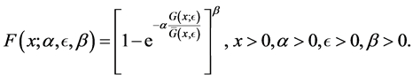
where  are scale parameters and
  is shape parameter.
2.2. PDF and Hazard Rate
If a random variable X has CDF in (3), then the corresponding probability density function is
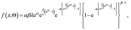 (4)
(4)
where 
A random variable  has survival function in the form
 (5)
(5)
The hazard rate function of  is given by
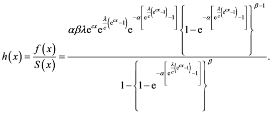 (6)
(6)
The cumulative distribution, probability density and hazard rate function of the OGE-G(Θ) are displayed is Figure 1, Figure 2 and Figure 3.
It is clear that the hazard function of the OGE-G distribution can be either decreasing, increasing, or of bathtub shape, which makes the distribution more flexible to fit different lifetime data set.
3. The Statistical Properties
In this section, we study some statistical properties of OGE-G, especially quantile, median, mode and moments.
3.1. Quantile and Median of OGE-G
The quantile of OGE-G(Θ) distribution is given by using
 (7)
(7)
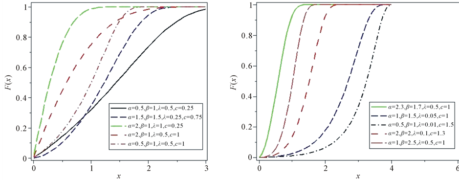
Figure 1. The CDF of various OGE-G distributions for some values of the parameters.
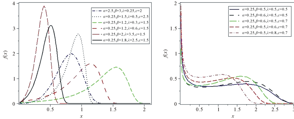
Figure 2. The pdf’s of various OGE-G distributions for some values of the parameters.
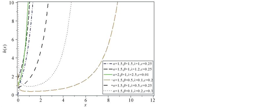
Figure 3. The hazard of various OGE-G distributions for some values of the parameters.
Substituting from (3) into (7),  can be obtained as
 (8)
(8)
The median of a random variable X that has probability density function  is a number
  such that

Therefore the median of OGE-G ( ) distribution can be obtained by setting q = 0.5 (50% quantile) in (8).
 (9)
(9)
3.2. The Mode of OGE-G
In this subsection, we will derive the mode of the OGE-G(Θ) distribution by deriving its pdf with respect to x and equal it to zero thus the mode of the OGE-G(Θ) distribution can be obtained as a nonnegative solution of the following nonlinear equation
 (10)
(10)
From Figure 2, the pdf for OGE-G distribution has only one peak. It is a unimodal distribution, so the above equation has only one solution. It is not possible to get an explicit solution of (10) in the general case. Numerical methods should be used such as bisection or fixed-point method to solve it.
3.3. The Moments
Moments are necessary and important in any statistical analysis, especially in applications. It can be used to study the most important features and characteristics of a distribution (e.g., tendency, dispersion, skewness and kurtosis). In this subsection, we will derive the rth moments of the OGE-G(Θ) distribution as infinite series expansion.
Theorem 1. If , where
 , then the rth moment of X is given by

Proof. The rth moment of the random variable X with pdf  is defined by
 (11)
(11)
Substituting from (4) into (11), we get
 (12)
(12)
Since  for
for , we have
 (13)
(13)
Substituting from (13) into (12), we obtain

Using the series expansion of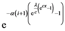 , we get

Using binomial expansion of , we get

Using series expansion of , we get

By using the definition of gamma function in the form

Thus we obtain the moment of OGE-G(Θ) as follows

This completes the proof.
4. The Order Statistic
Let  be a simple random sample of size n from OGE-G(Θ) distribution with cumulative distribution function
  and probability density function
  given by (3) and (4) respectively. Let
  denote the order statistics obtained from this sample. The probability density function of
  is given by
 (14)
(14)
where  and
and  are the pdf and cdf of OGE-G(Θ) distribution given by (3) and (4) respectively and
  is the beta function. Since
  for
for , we can use the binomial expansion of
  given as follows
 (15)
(15)
Substituting from (15) into (14), we have
 (16)
(16)
Substituting from (3) and (4) into (16), we obtain
 (17)
(17)
Thus  defined in (17) is the weighted average of the OGE-G distribution with different shape parameters.
5. Estimation and Inference
Now, we determine the maximum-likelihood estimators (MLE’s) of the OGE-G parameters.
5.1. The Maximum Likelihood Estimators
Let  be a random sample of size n from OGE-G(Θ), where
 , then the likelihood function
  of this sample is defined as
 (18)
(18)
Substituting from (4) into (18), we get

The log-likelihood function is given as follow
 (19)
(19)
The log-likelihood can be maximized either directly or by solving the nonlinear likelihood equations obtained by differentiating Equation (19) with respect to α, λ, c and β. The components of the score vector
 are given by
 (20)
(20)
 (21)
(21)
 (22)
(22)
 (23)
(23)
where 
The normal equations can be obtained by setting the above non-linear Equations (20)-(23) to zero. That is, the normal equations take the following form
 (24)
(24)
 (25)
(25)
 (26)
(26)
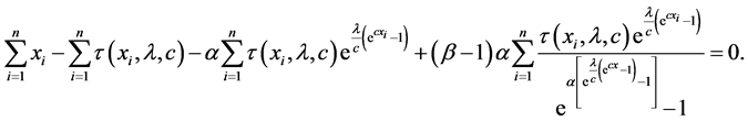 (27)
(27)
The normal equations do not have explicit solutions and they have to be obtained numerically. From Equation (24) the MLEs of β can be obtained as follows
 (28)
(28)
Substituting from (28) into (25), (26) and (27), we get the MLEs of α, λ, c by solving the following system of non-linear equations
 (29)
(29)
 (30)
(30)
 (31)
(31)
where 
These equations cannot be solved analytically and statistical software can be used to solve the equations numerically. We can use iterative techniques such as Newton Raphson type algorithm to obtain the estimate .
.
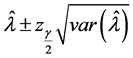
5.2. Asymptotic Confidence Bounds
In this subsection, we derive the asymptotic confidence intervals of the unknown parameters α, λ, c, β when ,
,  ,
,  and
and . The simplest large sample approach is to assume that the MLEs (α, λ, c, β) are approximately multivariate normal with mean (α, λ, c, β) and covariance matrix
 , where
  is the inverse of the observed information matrix which defined as follows
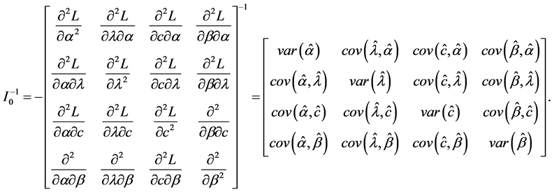 (32)
(32)
The second partial derivatives included in  are given as follows

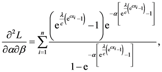


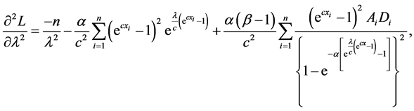


where


The asymptotic  confidence intervals of α, λ, c and β are
 ,
,  ,
,  and
and  respectively, where
  is the upper
  percentile of the standard normal distribution.
6. Data Analysis
In this section we perform an application to real data to illustrate that the OGE-G can be a good lifetime model, comparing with many known distributions such as the Exponential, Generalized Exponential, Gompertz, Generalized Gompertz and Beta Gompertz distributions (ED, GE, G, GG, BG), see [4] [6] [10] [11] .
Consider the data have been obtained from Aarset [9] , and widely reported in some literatures, see [3] [4] [12] -[15] . It represents the lifetimes of 50 devices, and also, possess a bathtub-shaped failure rate property, Table 1.
Based on some goodness-of-fit measures, the performance of the OGE-G distribution is compared with others five distributions: E, GE, G, GG, and BG distributions. The MLE's of the unknown parameters for these distributions are given in Table 2 and Table 3. Also, the values of the log-likelihood functions (-L), the statistics K-S (Kolmogorov-Smirnov), AIC (Akaike Information Criterion), the statistics AICC (Akaike Information Citerion with correction) and BIC (Bayesian Information Criterion) are calculated for the six distributions in order to verify which distribution fits better to these data.
Based on Table 2 and Table 3, it is shown that OGE-G (α, λ, c, β) model is the best among of those distributions because it has the smallest value of (K-S), AIC, CAIC and BIC test.
Substituting the MLE’s of the unknown parameters α, λ, c, β into (32), we get estimation of the variance covariance matrix as the following
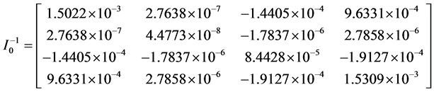 The approximate 95% two sided confidence intervals of the unknown parameters α, λ, c and β are
 ,
,  ,
,  and
and , respectively.To show that the likelihood equation have unique solution, we plot the profiles of the log-likelihood function of α, λ, β and c in Figure 4 and Figure 5.

Table 1. The data from Aarset [9] .
Table 2. The MLE’s, log-likelihood for Aarset data.
Table 3. The AIC, CAIC, BIC and K-S values for Aarset data.
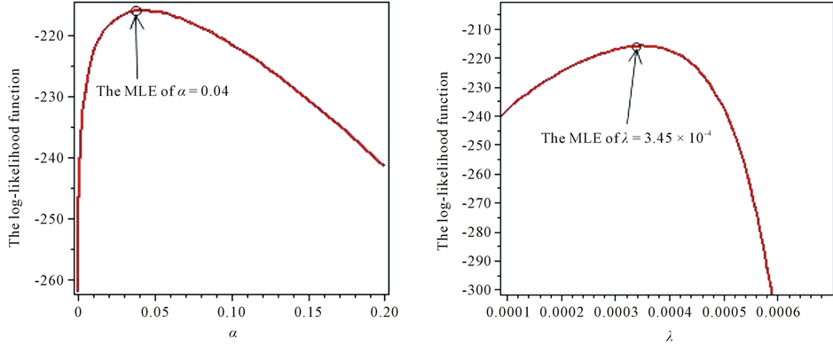
Figure 4. The profile of the log-likelihood function of α, λ.
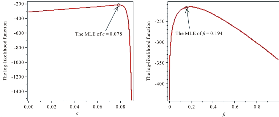
Figure 5. The profile of the log-likelihood function of c, β.
The nonparametric estimate of the survival function using the Kaplan-Meier method and its fitted parametric estimations when the distribution is assumed to be ED, GED, GD, GGD and OGE-GD are computed and plotted in Figure 6.
Figure 7, gives the form of the hazard rate for the ED, GED, GD, GGD, BGD and OGE-GD which are used to fit the data after replacing the unknown parameters included in each distribution by their MLE.
7. Conclusion
In this paper, we propose a new model, called the Odd Generalized Exponential-Gompertz (OGE-G) distribution and studied its different properties. Some statistical properties of this distribution have been derived and discussed. The quantile, median, mode and moments of OGE-G are derived in closed forms. The distribution of the order statistics is discussed. Both point and asymptotic confidence interval estimates of the parameters are derived using the maximum likelihood method and we obtained the observed Fisher information matrix. We use application on set of real data to compare the OGE-G with other known distributions such as Exponential (E), Generalized Exponential (GE), Gompertz (G), Generalized Gompertz (GG) and Beta-Gompertz (BG). Applications on set of real data showed that the OGE-G is the best distribution for fitting these data sets compared with other distributions considered in this article.
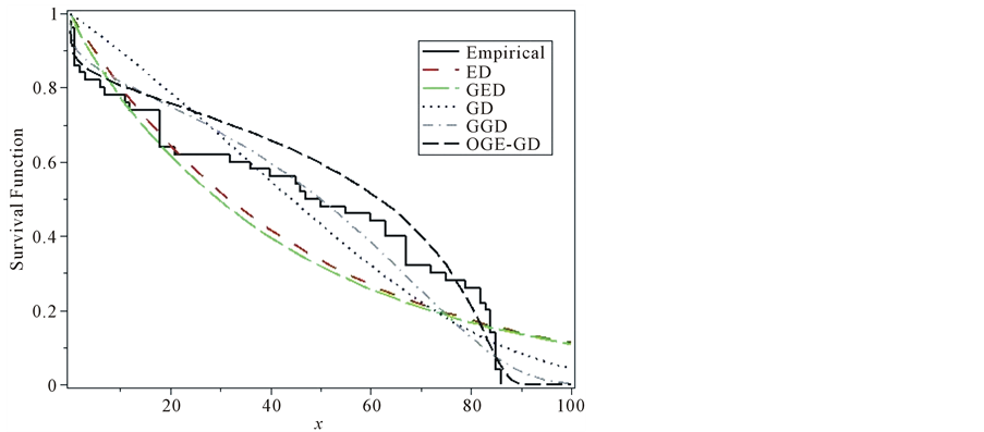
Figure 6. The Kaplan-Meier estimate of the survival function.
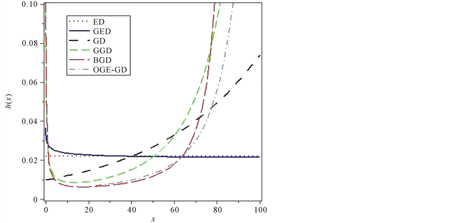
Figure 7. The Fitted hazard rate function for the data.
Acknowledgments
The authors are grateful to the anonymous referee for a careful checking of the details and for helpful comments that improved this paper.
Cite this paper
M. A.El-Damcese,AbdelfattahMustafa,B. S.El-Desouky,M. E.Mustafa, (2015) The Odd Generalized Exponential Gompertz Distribution. Applied Mathematics,06,2340-2353. doi: 10.4236/am.2015.614206
References
- 1. Pollard, J.H. and Valkovics, E.J. (1992) The Gompertz Distribution and Its Applications. Genus, 48, 15-28.
- 2. Marshall, A.W. and Olkin, I. (2007) Life Distributions. Structure of Nonparametric, Semiparametric and Parametric Families. Springer, New York.
- 3. Abu-Zinadah, H.H. and Aloufi, A.S. (2014) Some Characterizations of the Exponentiated Gompertz Distribution. International Mathematical Forum, 9, 1427-1439.
- 4. El-Gohary, A., Alshamrani, A. and Al-Otaibi, A.N. (2013) The Generalized Gompertz Distribution. Applied Mathematical Modelling, 37, 13-24.
http://dx.doi.org/10.1016/j.apm.2011.05.017 - 5. Eugene, N., Lee, C. and Famoye, F. (2002) Beta-Normal Distribution and Its Applications. Communications in Statistics-Theory and Methods, 31, 497-512.
http://dx.doi.org/10.1081/STA-120003130 - 6. Jafari, A.A., Tahmasebi, S. and Alizadeh, M. (2014) The Beta-Gompertz Distribution. Revista Colombiana de Esta-distica, 37, 141-158.
http://dx.doi.org/10.15446/rce.v37n1.44363 - 7. Mudholkar, G.S. and Srivastava, D.K. (1993) Exponentiated Weibull Family for Analyzing Bathtub Failure Data. IEEE Transactions on Reliability, 42, 299-302.
http://dx.doi.org/10.1109/24.229504 - 8. Tahir, M.H., Cordeiro, G.M., Alizadeh, M., Mansoor, M., Zubair, M. and Hamedani, G.G. (2015) The Odd Generalized Exponential Family of Distributions with Applications. Journal of Statistical Distributions and Applications, 2, 1-28.
http://dx.doi.org/10.1186/s40488-014-0024-2 - 9. Aarset, M.V. (1987) How to Identify a Bathtub Hazard Rate. IEEE Transactions on Reliability, 36, 106-108.
http://dx.doi.org/10.1109/TR.1987.5222310 - 10. Gupta, R.D. and Kundu, D. (2007) Generalized Exponential Distribution: Existing Results and Some Recent Developments. Journal of Statistical Planning and Inference, 137, 3537-3547.
http://dx.doi.org/10.1016/j.jspi.2007.03.030 - 11. Gupta, R.D. and Kundu, D. (2001) Generalized Exponential Distribution: Different Method of Estimations. Journal of Statistical Computation and Simulation, 69, 315-337.
http://dx.doi.org/10.1080/00949650108812098 - 12. Lenart, A. (2014) The Moments of the Gompertz Distribution and Maximum Likelihood Estimation of Its Parameters. Scandinavian Actuarial Journal, 2014, 255-277.
http://dx.doi.org/10.1080/03461238.2012.687697 - 13. Nadarajah, S. and Kotz, S. (2006) The Beta Exponential Distribution. Reliability Engineering & System Safety, 91, 689-697.
http://dx.doi.org/10.1016/j.ress.2005.05.008 - 14. Pasupuleti, S.S. and Pathak, P. (2010) Special Form of Gompertz Model and Its Application. Genus, 66, 95-125.
- 15. Gupta, R.D. and Kundu, D. (1999) Generalized Exponential Distribution. Australian and New Zealand Journal of Statistics, 41, 173-188.
http://dx.doi.org/10.1111/1467-842X.00072