Modern Economy
Vol.5 No.1(2014), Article ID:42336,7 pages DOI:10.4236/me.2014.51012
Analysis of the Goods Market and Money Market Equilibrium in a Developing Country
1School of Business, Wa Polytechnic, Wa, Upper West Region, Ghana
2GIMPA Business School, Ghana Institute of Management and Public Administration, Achimota, Accra, Ghana
Email: nsahbaba@yahoo.com, hspgh@yahoo.com
Copyright © 2014 Insah Baba, Ofori-Boateng Kenneth. This is an open access article distributed under the Creative Commons Attribution License, which permits unrestricted use, distribution, and reproduction in any medium, provided the original work is properly cited. In accordance of the Creative Commons Attribution License all Copyrights © 2014 are reserved for SCIRP and the owner of the intellectual property Insah Baba, Ofori-Boateng Kenneth. All Copyright © 2014 are guarded by law and by SCIRP as a guardian.
Received December 4, 2013; revised January 4, 2014; accepted January 11, 2014
KEYWORDS
IS-LM; Simultaneous Equation; Real Interest Rate; Real Money Balances
ABSTRACT
The relationship between interest rate, real money balances and real output may be explored in an IS-LM framework. The objective of this study is to explore the connection between real interest rate, GDP and real money balances. It also empirically tests for the nature and existence of the IS-LM framework in Ghana. Employing a simple IS-LM framework, the Two Stage Least Squares (TSLS) estimation technique is used for the analysis. The main contribution of this paper is the use of a simultaneous equation framework to investigate interest rate and GDP growth determinants. This is imperative since interest rate is both an explanatory and an explained variable. The results indicated that real money balances exerted a negative but significant influence on real interest rate. The growth rate of GDP had a dominant influence on real interest rate. On the other hand, investment expenditure exerted significant and positive influence on GDP growth. Meanwhile, as informed by economic theory, interest rate changes had a negative and significant influence on GDP growth. The study recommends the role of monetary policy and economic growth in exchange rate management. Also, policy focus should be on interest rate since interest rate is seen in this study as a stronger driver of economic growth in Ghana compared with investment expenditure.
1. Introduction
The Investment Saving-Liquidity Preference Money Supply (IS-LM) model is a macroeconomic tool that demonstrates the relationship between interest rates and real output in the goods and services market and the money market. It is a combination of the goods market and money market equilibriums. This aggregate model describes a general equilibrium situation in the Macroeconomy. The IS-LM model is based on the assumption of a fixed price level. This means that the general price level will not suddenly adjust when economic conditions change. Suppose an increase in the demand. Given the supply, this increase in the demand should result in an increase in the price level (and in the quantity exchanged in the market). The period which it stays unchanged is the short run.
The Keynesian cross diagram provides a vital tool for explaining the IS-LM model. The Keynesian cross shows how the spending plans of households, firms, and the government determine output. From economic theory, there is a strong relationship between the interest rate and planned investment. This relationship between interest rate and planned investment is explainable. Since interest rate is the cost of borrowing to finance investment, an increase in the interest rate reduces planned investment. On the other side, investment is one of the components of aggregate output and thus, the reduction in planned investment shifts the planned-expenditure function downward. The shift in the planned expenditure function causes the level of output to fall [1]. The reverse holds for a decrease in interest rate.
The IS-LM model was first developed by John Hicks in 1937 [2]. This was as an attempt to portray the central ideas of Keynes’s General Theory. As suggested by Tobin [3,4], the IS-LM model provides a common framework that economists use to discuss macroeconomic policy. The IS-LM model allows for the investigation of the role of monetary policy and fiscal policy in an economy. An increase in the money supply shifts the LM curve downward and to the right, lowering interest rates and raising equilibrium national income. Also, an exogenous decrease in liquidity preference leads to downward shifts of the LM curve and thus an increase in income and a corresponding decrease in interest rates. Changes in these variables in the opposite direction shift the LM curve in the opposite direction. On the other hand, exogenous increases in investment spending (i.e., for reasons other than interest rates or income), shift the IS curve rightward resulting from consumer spending. This also raises both equilibrium income and the equilibrium interest rate. Of course, changes in these variables in the opposite direction shift the IS curve in the opposite direction.
Existing studies have investigated the determinants of interest rate as a monetary policy tool and also its impact on economic growth. Single equation and atheoretic techniques of estimation have been used to investigate the factors that influence interest rates. These studies do not take into consideration the presence of endogenous explanatory variables. That is, some predetermined variables may also be explained variables. The above informs the analysis of the determinants of interest rate and that of real GDP in a manner that would take care of the jointly determined variables. This would better inform policy due to the interdependence of phenomena.
The main objective of this study is to explore the connection between real interest rate, GDP and real money balances. A plethora of studies have investigated the determinants of interest rate and GDP growth in single equation contexts. However, this study attempts to investigate the relationships in a simultaneous equation model which is deemed appropriate. It will also empirically test for the nature, existence and the intuition of the IS-LM model for a developing economy of the IS-LM framework.
The rest of the study is arranged as follows. The next is Section 2 which covers a review of literature. This is followed by the methodology adopted for the study in Section 3. Section 4 presents findings from the study and Section 5 is the conclusion of the study.
2. Literature Review
According to the classical theory, interest, in real terms, is the reward for the productive use of capital, which is equal to the marginal productivity of physical capital. This theory posits that interest is the price paid for not spending the income. But according to Keynes, interest is not the reward for not spending, but is the price paid for not hoarding. This theory is based on equality of savings and investment. The equality of savings and investment is brought by changes in rate of interest. However as noted by Keynes, the changes in level of income bring equality between saving and investment. For example, when rate of interest falls, investment increases and when investment increases, the level of income increases. When level of income increases, savings also increase. Since physical capital is purchased with monetary funds in a money economy, the rate of interest is taken to be the annual rate of return over money capital invested in physical capital assets. Keynes further asserted that the true classical theory of interest rate is the savings investment theory. This theory holds the proposition based on the general equilibrium theory that the rate of interest is determined by the intersection of the demand for and supply of capital.
The Keynesian liquidity preference theory is a stock concept that determines the interest rate by the demand for and supply of money. This theory is a stock analysis because it takes the supply of money as given in the short run and determines the interest rate by liquidity preference or demand for money. The rate of interest here is seen as a pure monetary phenomenon. Another theory of interest rate is the loanable funds theory. This theory on the other hand is a flow concept that determines the interest rate by the demand for and supply of loanable funds. It involves the linking of interest rates with savings, dishoarding and bank money on the supply side. This work is however anchored on the Keynesian theory.
There have been several studies that attempt to translate modern work into the IS/LM framework, such as we see in the work of [5-7]. However, the foundation of their models is in dynamic general equilibrium theory. Furthermore, the translation into IS-LM is not central to their analysis. Their translation gives policy-oriented economists a way of relating their conclusions to an IS-LM framework. A presentation of the use of the IS-LM by Klein [8] shows how IS-LM would be presented empirically.
In their paper on the IS-LM model, Josheski [9] introduced a time series model. They used a standard vector autoregression (VAR) and a vector error correction mechanism (VECM). The variables that were estimated were logarithm of real GDP, interbank interest rate and real monetary base. The VECM mechanism showed that if the system is in disequilibrium there would be a downward alteration in these variables. Blanchard & Fisher [10] found the LM curve to be consistent with the demand for money. They also concluded that the IS function was an analysis of savings and investment under uncertainty.
Abayomi and Adebayo [11] in their paper analyzed the determinants of interest rate in Nigeria within the framework of a Vector Error Correction Model (VECM). The results based on normalisation of the restricted VAR system in respect of the Treasury Bill rate and real GDP revealed that real money supply and expected foreign returns exert a negative and significant long-run influence on both the Treasury Bill Rate and domestic output. Further, Edwards and Khan [12] in a study of the behaviour of nominal interest rates in a small semi-open economy found evidence that excess supply of real money exerted significant negative pressure on nominal interest rates.
The role of investments in economic growth has been much researched. According to Solow [13] the larger the investment and saving rate are the more cumulative capital per worker is produced. Similarly, as others have noted, exports and investments are the main determinants of economic growth Tyler [14].
New growth theories stress the importance of investments among others in the long-run economic growth of any economy. Theoretically, the channels and linkages are that the gross capital formation affects the economic growth. This effect is achieved directly and indirectly. Directly, this is achieved by increasing the physical capital stock in domestic economy Plossner [15]. Indirectly, it is achieved by promoting the technology [16].
Udoka and Anyingang [17] investigating the determinants of GDP noted that the estimated coefficient for interest rate is negative, indicating that there exist an inverse relationship between interest rate and GDP. This means that when interest rate increases GDP will also decrease. The result is in order with economic theory. The result was also statistically significant at 5 percent level of significance.
As noted by Κhan and Kumar [12] the effects of private and public investments on economic growth differ significantly. He noted that private investment was more productive than public investment. Other studies have confirmed that public investments on infrastructure have an important positive effect on economic growth [18,19]. Evaluating public investments on transportation and communications, Εasterly and Rebelo [20] noted that they are positively correlated to economic growth, while there were negative effects of public investments of state-owned businesses on economic growth.
From the review of the literature so far, studies have ignored the joint determination and interdependence of macroeconomic variables. It is thus imperative to consider the analysis of interest and real GDP determinants using a simultaneous equation model.
3. Theoretical Framework and Methodology
3.1. Model and Methodology
A closed economy without public sector is considered. The investment—saving (IS) function represents equilibrium in the goods market where aggregate output equals aggregate demand. For the IS function, the independent variable is the interest rate and the dependent variable is the level of income. Furthermore, the IS function can be said to represent the equilibria where total private investment equals total saving, In equilibrium, all spending is desired or planned; there is no unplanned inventory accumulation. The level of real GDP (Y) is determined along this trajectory for each interest rate.
For the liquidity preference-money supply function, the independent variable is income and the dependent variable is the Interest rate. The LM curve shows the combinations of interest rates and levels of real income for which the money market is in equilibrium. It is an upward-sloping curve representing the role of finance and money. The assumption is that the money supply is a fixed quantity in the short-run and is determined by the government. The demand for money is a function of prices, income/output, and the real interest rate. The theory upon which the model is formulated is the IS-LM framework. Generally, the model is formulated as:
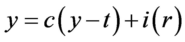 (1)
(1)
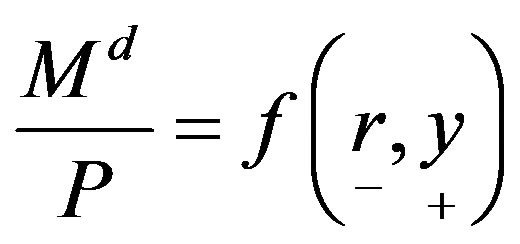 (2)
(2)
where y is output, t is tax revenue, r is the real interest rate,  is the desired consumption and
  is the desired investment. Also,
  is real money balances and r is the real interest rate. The minus sign says that real money balances are negatively related to interest rates and the plus sign says that real money balances are positively related to income.
3.2. Econometric Specification of the Model
From theory and the literature reviewed, the structural model to be investigated in a log-log form set up as follows:
 (3)
(3)
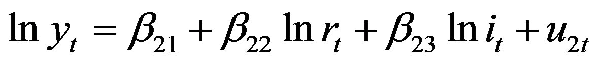 (4)
(4)
where rt denotes the real interest rate, mt is the real money stock. In Equation (4), yt is GDP and it is investment expenditure.
Each equation in the structural model is identified since lnyt and lnrt are jointly endogenous variables. Both equations are over identified since in either case there are more instruments than the endogenous regressors. The instruments used are lnmt, lnit and lnmt (−1). The endogenous regressors are lnrt and lnyt. Ordinary least squares estimations would lead to simultaneity bias and inconsistent estimates. The over identification justifies the use of the Two-stage Least Squares (TSLS) estimation technique. The reduced form cannot also be used here to get the exact estimation indirectly. The reason is that obtaining the original postulated parameters would require more than one solution.
The ISLM model forms the theoretical basis for the structure of the model. The eviews package makes it possible to estimate the TSLS regression directly without resorting to the reduced form estimate or the OLS twostage regression methods. This makes possible the estimation of the structural form of the model as informed by economic theory.
The choice of instrument specification is not arbitrary but depends on the variables in the system of equations. The instruments used are the constant, money supply, investment and a one year lag of money supply.
This model is estimated as a simultaneous model to take care of interdependence of phenomena. Interest rate is seen in the system of equations as both an explained and an explanatory variable. This is modeled using a Two Stage Least Square (TSLS) regression technique. This estimation technique suits the analysis because multiple regression models are adjusted by the Least Squares method. This minimizes the sum of the squares of the prediction errors. Alternative estimation techniques are the Bayesian and the Maximum Likelihood methods. The maximum likelihood approach is not appropriate because it only makes the likelihood of the sample maximum. The term least squares describe a frequently used approach to solving over determined or inexactly specified systems of equations in an approximate sense. Instead of solving the equations exactly, we seek only to minimize the sum of the squares of the residuals.
The minimization process reduces the over determined system of equations formed by the data to a sensible system. Time series properties of stationarity were investigated using the Augmented Dickey-Fuller (ADF), Phillips-Perron (PP) and the Kwiatkowski-Phillips-SchmidtShin (KPSS) test.
In the model, lnr is the log of real interest rate. The variable lny is growth rate of the economy using GDP. The log of real money balances is lnm measured using M2. The variable lni is investment expenditure captured by expenditure on capital items only.
4. Empirical Findings
4.1. Time Series Characteristics of the Variables Used in the Model
The time series characteristics of the variables using the three tests reveal that most of the variables are stationary with intercept. This captures the nonzero mean under the alternative hypothesis. However, many of the variables are not stationary with a constant and deterministic time trend. This also captures the deterministic trend under the alternative. The variables may therefore be regarded as stationary and do not require differencing. These results are shown in Table 1 (see Appendix).
4.2. Discussion of Model’s Results
The estimated LM function showed that real money balances and GDP growth have significant effects on interest rate as informed by economic theory. The interest rate elasticity with respect to real money balances is 3.21. This elasticity is large, negative and significant at the 1% significance level. This outcome supports existing literature [21,22] who noted that real money supply exerted a negative and significant long-run influence on both the Treasury Bill Rate and domestic output. The implication of this inverse elasticity is that a percentage increase in real money balances would result in a 3.21 percentage decrease in the interest. The reverse holds as well.
Further, GDP growth has a bigger elasticity of 4.29. However, this relation is positive and significant at the 5% significance level. This means that a percentage increase in real GDP would result in a 3.21 percentage increase in the interest and vice versa. Using the Wald test, the low probability value and level of significance of the F-statistic indicates that the coefficients are statistically different from zero. The very small adjusted R-squared suggests that there are variables missing from the equation and does not affect the validity and reliability of the estimates.
Since it is established that the models are identified, we test the exogeneity of the instruments using the overidentification test. The null hypothesis is that all the Instrumental Variables are exogenous. The J-statistic is 0.000000. This presupposes that we cannot reject the null hypothesis. Alternatively, the Craig-Donald F-statistic is 32.7 and by convention we cannot reject the null hypothesis since it is greater than 10. Further, the associated Stock-Yugo critical value for this F-value is 16.38 at the 10% significance level. This analysis further indicates that we cannot reject the null hypothesis. That means there is some asymptotic efficiency gain from including them as instruments. These results are shown in Table 2.
On the other hand, results of the IS equation also indicated that real interest rate exerted a stronger influence on GDP growth than that of investment expenditure. All coefficients were significant at the 1% level of significance. The GDP growth elasticity with respect to interest rate was a negative value of 1.24. This outcome supports existing literature such as Udoka and Anyingang [23] who asserted that there existed inverse relationship between interest rate and GDP growth. The interpretation is that the responsiveness of a unit increase (decrease) in real interest rate to GDP growth is 1.24. However this relationship is an inverse one. Meanwhile, the elasticity of GDP growth with respect to investment expenditure is positive and weaker at 0.88. This outcome also supports existing literature [18-20]. The meaning is that rate of change of GDP growth with respect to investment expenditure is 0.88. When investment expenditure changes by one unit, GDP changes by 0.88 which is less responsive. The adjusted R-squared is high and the Wald test also indicates that the results are statistically different from zero.
Testing the exogeneity of the instruments, the J-statistic is 0.870724 and not statistically significant. The Craig-Donald F-statistic is 3.768 and by convention we can reject the null hypothesis. To add, the Stock-Yugo critical value for this F-value is 19.93 at the 10% significance level. These indicate that we can further reject the null hypothesis of instrument exogeneity. Notwithstanding, instrument exogeneity is only a measure of asymptotic efficiency gain and not the explanatory power of the model. The results are shown in Table 3.
5. Conclusion
This study used annual time series data from 1980 to 2012. The study among others sought to explore the connection between real interest rate, GDP and real money balances. A simultaneous equation framework was employed for the study. The theoretical basis for the estimation was based on the IS-LM model. The results from the LM analysis revealed that the interest rate elasticity with respect to real money balances was large, negative and significant at the 1% significance level. Meanwhile, the elasticity with respect to GDP is positive and significant at the 5% significance level. The GDP growth elasticity with respect to interest rate was negative and significant at the 1% level of significance.
On the other hand, results of the IS equation also indicated that real interest rate exerted a stronger influence on GDP growth than that of investment expenditure. All coefficients were significant at the 1% level of significance. The GDP growth elasticity with respect to interest rate was negative whereas that of investment expenditure was positive. The study thus recommends the role of monetary policy and economic growth in exchange rate management. Also, interest rate is seen here as a stronger driver of economic growth in Ghana compared with investment expenditure.
REFERENCES
- G. N. Mankiw, “Macroeconomics,” 5th Edition, Worth Publishers, 2003, pp. 257-178.
- J. R. Hicks, “Mr. Keynes and the ‘Classics’,” Econometrica, Vol. 5, No. 2, 1937, pp. 147-159.
- T. James, “Asset Accumulation and Economics Activity,” Basil Blackwell, Oxford, 1980.
- S. Robert, “Mr. Hicks and the Classics,” Oxford Economic Papers, Vol. 36, 1984.
- B. McCallum and N. Edward, “An Optimizing IS-LM Specification for Monetary Policy and Business Cycle Analysis,” Journal of Money, Credit and Banking, Vol. 31, No. 3, 1999, pp. 296-316. http://dx.doi.org/10.2307/2601113
- T. Yun, “Nominal Price Rigidity, Money Supply Endogeneity, and Business Cycles,” Journal of Monetary Economics, Vol. 37, No. 2, 1996, pp. 345-370. http://dx.doi.org/10.1016/S0304-3932(96)90040-9
- J. G. Clarida and M. Gertler, “The Science of Monetary Policy: A New Keynesian Perspective,” Journal of Economic Literature, Vol. 37, No. 4, 1999, pp. 1661-1707. http://dx.doi.org/10.1257/jel.37.4.1661
- L. Klein, “The IS-LM Model: Its Role in Macroeconomic,” In: W. Young and B. Z. Zilberfarb, Eds., IS-LM and Modern Macroeconomics, Kluwer Academic Publishers, Boston and London, 2000. http://dx.doi.org/10.1007/978-94-010-0644-6_11
- D. Josheski, “IS-LM Model for US Economy: Testing in JMULTI,” MPRA, Paper No. 34024, 2011. http://mpra.ub.uni-muenchen.de/34024/
- O. A. Blanchard and S. Fischer, “Lectures on Macroeconomics,” MIT Press, Cambridge, 1989.
- T. O. Abayomi and M. S. Adebayo, “Determinants of Interest Rates in Nigeria: An Error Correction Model,” Journal of Economics and International Finance, Vol. 2, No. 12, 2010, pp. 261-271.
- M. Khan and M. Kumar, “Public and Private Investment and the Growth Process in Developing Countries,” Oxford Bulletin of Economics and Statistics, Vol. 59, No. 1, 1997, pp. 69-88.
- R. Solow, “A Contribution to the Theory of Economic Growth,” Quarterly Journal of Economics, Vol. 70, No. 1, 1956, pp. 65-94.
- W. Tyler, “Growth and Export Expansion in Developing Countries: Some Empirical Evidence,” Journal of Development Economics, Vol. 9, No. 1, 1981, pp. 121-310.
- C. Plossner, “The Search for Growth in Policies for LongRun Economic Growth,” Federal Reserve Bank of Kansas City, Kansas City, 1992.
- R. Levine and D. Renelt, “A Sensitivity Analysis of CrossCountry Growth Regressions,” American Economic Review, Vol. 82, No. 4, 1992, pp. 942-963.
- C. O. Udoka and R. Anyingang, “The Effect of Interest Rate Fluctuation on the Economic Growth of Nigeria, 1970-2010,” International Journal of Business and Social Science, Vol. 3, No. 20, 2012, pp. 295-303.
- M. Knight, N. D. Loyaza and Villanueva, “Testing the Neoclassical Theory of Economic Growth,” IMF Staff Papers, Vol. 40, No. 3, 1993, pp. 512-541. http://dx.doi.org/10.2307/3867446
- M. Nelson and R. Singh, “The Deficit Growth Connection: Some Recent Evidence from Developing Countries,” Economic Development and Cultural Change, Vol. 43, No. 1, 1994, pp. 167-191. http://dx.doi.org/10.1086/452140
- W. Easterly and S. Rebelo, “Fiscal Policy and Economic Growth: An Empirical Investigation,” Journal of Monetary Economics, Vol. 32, No. 3, 1993, pp. 417-458. http://dx.doi.org/10.1016/0304-3932(93)90025-B
- T. O. Abayomi and M. S. Adebayo, “Determinants of Interest Rates in Nigeria: An Error Correction Model,” Journal of Economics and International Finance, Vol. 2, No. 12, 2010, pp. 261-271.
- S. Edwards and M. S Khan, “Interest Rate Determination in Developing Countries: A Conceptual Framework,” IMF Staff Paper, 1995, pp. 377-403.
- C. O. Udoka and R. Anyingang, “The Effect of Interest Rate Fluctuation on the Economic Growth of Nigeria, 1970- 2010,” International Journal of Business and Social Science, Vol. 3, No. 20, 2012, pp. 295-303.
Appendix
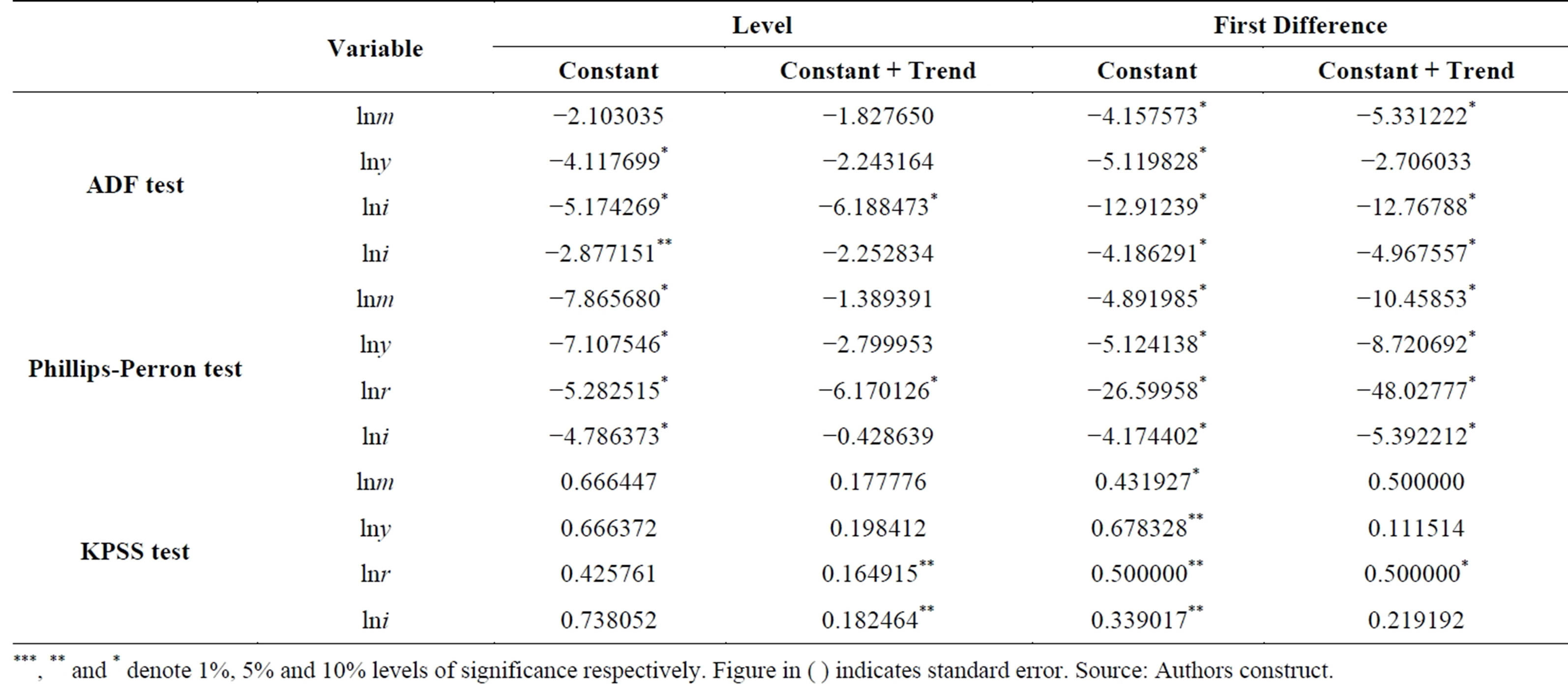
Table 1. Results of unit root tests with and without trend.
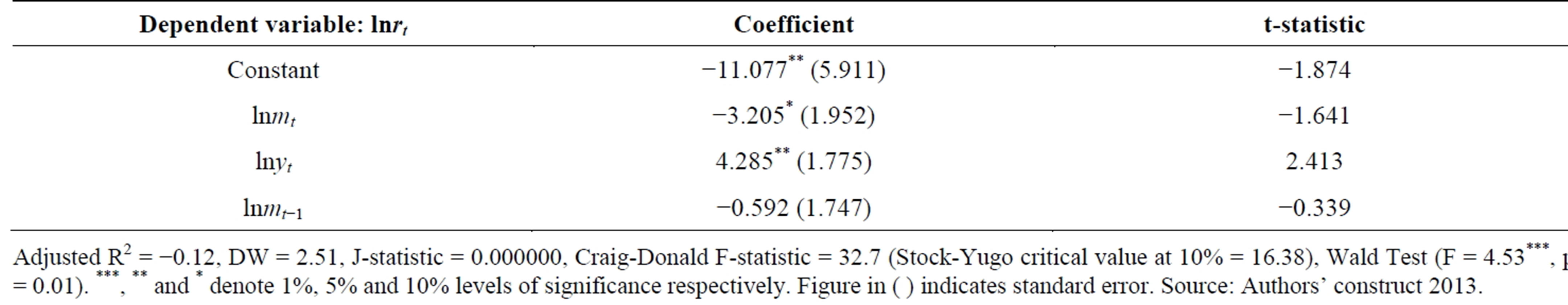
Table 2. Two stage least squares estimation results-LM Function Intruments: lnm, lni and lnm.
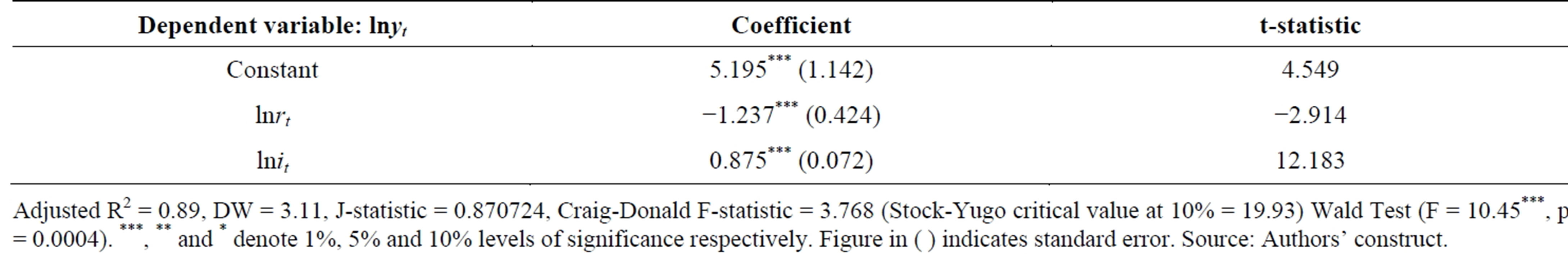
Table 3. Two stage least squares estimation results-IS Function Instruments: lnm, lni and lnm.