Journal of Environmental Protection
Vol. 3 No. 9A (2012) , Article ID: 22975 , 15 pages DOI:10.4236/jep.2012.329139
Comparing the Adequacy of Some Non-Homogeneous Poisson Models to Estimate Ozone Exceedances in Mexico City
![]()
1Faculdade de Medicina de Ribeirão Preto, Universidade de São Paulo, São Paulo, Brazil; 2Facultad de Ciencias, Universidad Nacional Autónoma de México, México City, México; 3Instituto de Matemáticas, Universidad Nacional Autónoma de México, México City, México.
Email: achcar@fmrp.usp.br, *jbarrios@ciencias.unam.mx, eliane@math.unam.mx
Received June 30th, 2012; revised July 28th, 2012; accepted August 29th, 2012
Keywords: MCMC algorithms; non-homogeneous Poisson models; change-points; ozone air pollution; Mexico City
ABSTRACT
We consider some non-homogeneous Poisson models to estimate the mean number of times that a given environmental threshold of interest is surpassed by a given pollutant. Seven different rate functions for the Poisson processes describing the models are taken into account. The rate functions considered are the Weibull, exponentiated-Weibull, and their generalisation the Beta-Weibull rate function. We also use the Musa-Okumoto, the Goel-Okumoto, a generalised GoelOkumoto and the Weibull-geometric rate functions. Whenever thought justifiable, the model allowing the presence of change-points is also going to be considered. The different models are applied to the daily maximum ozone measurements data provided by the monitoring network of the Metropolitan Area of Mexico City. The aim is to compare the adjustment of different rate functions to the data. Even though, some of the rate functions have been considered before, now we are applying them to the same data set. In previous works they were used in different data sets and therefore a comparison of the adequacy of those models were not possible. The measurements considered here were obtained after a series of environmental measures were implemented in Mexico City. Hence, the data present a different behaviour from that of earlier studies.
1. Introduction
Inhabitants of large cities throughout the world may present health problems related to high levels of pollution. Among the pollutants affecting the health of those inhabitants we have ozone. When exposed to ozone concentration levels above 0.11 parts per million (0.11 ppm), a very sensitive part of the population may present a deterioration in their health (see for instance [1-8]).
In the case of Mexico City, even though the air quality has improved considerably in the past twenty years, ozone still presents high concentration levels. The Mexican environmental standard for ozone is 0.11 ppm [9] and individuals should not be exposed to it, on average, for a period of one hour or more. That standard is frequently surpassed by ozone concentration in Mexico City. Even though the Mexican standard is 0.11 ppm, the threshold used to declare an emergency alert in Mexico City is 0.2 ppm (see www.sma.df.gob.mx). This threshold is seldom surpassed. Throughout this work we are going to take 0.17 ppm as our threshold. We do so, because that is an intermediate value between 0.11 ppm and 0.2 ppm. Also, we would like to know how emergency alert situations would be if 0.17 ppm, instead of 0.2 ppm, was the threshold considered to declare them in Mexico City. That is important since we could have an idea of how frequent emergency alerts would be declared if 0.17 ppm were considered by the environmental authorities as the threshold instead of 0.2 ppm. Using that information it is possible to plan the lowering of environmental threshold in such a way that little by little the Mexican environmental standard would be approached without causing too much disruption in the population’s activities. The theoretical threshold is analysed and prediction on the number of environmental alerts that would be declared can be made.
There are several works in the literature dealing with the problem of modelling the behaviour of pollutants in general and in particular ozone. Those works study the problem from different points of view. They also use a great variety of methodologies to analyse the different aspects of the problem. Some of the many works studying ozone behaviour are [10-13] considering extreme value theory; [14-18] using time series analysis; [19,20] considering Markov chain models; [21-23] using stochastic volatility models; and [24] with an analysis of the behaviour the maximum measurements of ozone with an application to the data from Mexico City. [25,26] present studies that analyse the impact on air quality of the driving restriction imposed in Mexico City.
In this work the interest resides in studying the problem from the point of view of estimating the mean number of times that the concentration surpasses a given threshold. In order to study this problem, Poisson processes may be used. Among the works using that methodology we may quote [27,28] using homogeneous Poisson processes and [29-32] using non-homogeneous Poisson processes.
The non-homogeneous approach is going to be followed here as well. We consider several rate functions for the Poisson process modelling the problem. One of the aims here is to compare the fit of different rate functions, considered in the literature, to the ozone data from Mexico City obtained after a series of environmental measures were taken to decrease air pollution levels. Even though some of the rate functions considered here were taken into account in previous works, usually they were applied to different data sets. Hence, it was not possible to compare their performance when applied to the same set of measurements. That was so because depending on the dataset the rate function that best fitted the data would change. Therefore, using the data obtained after the series of environmental measures were implemented would give a more precise information on how the pollutant is behaving in more recent times and also on the impact that those measures might have had on the ozone behaviour. Hence, in here we are going to consider the many different rate functions and compare their performance when using the more recent ozone measurements. When the best Poisson model is selected for the data considered here, then we may perform inference about the mean time between surpassings of the 0.17 ppm threshold and also about the probability of a certain number of exceedances in a time interval of interest. Another aim here is to present the code in R when some of the functions are used so the readers can use them in their own studies if the situation arises.
This work is divided as follows. Section 2 presents the different non-homogeneous Poisson models considered here. In Section 3 we have the Bayesian formulation of the problem. An application of the results to ozone measurements from Mexico City is given in Section 4. Finally, in Section 5, a discussion of the results presented here is given. Some of the computer programmes used in the estimation of the parameters can be obtained from https://sites.google.com/site/jmbarrios/recursos/result-reports-for-jep.
2. The Poisson Models
The mathematical description of the models considered here is given as follows. Assume that a given environmental threshold is surpassed by a pollutant’s concentration according to a non-homogeneous Poisson process with some rate function ,
, . Hence, if
  denotes the non-homogeneous Poisson process recording the number of times that the pollutant surpasses the threshold of interest, then
  indicates the number of times that exceedances occurred in the time interval
 ,
, . Let
. Let  denote the mean function of the Poisson process
 . Hence, for
  and
and , we have that
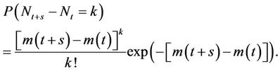
We consider several parametric forms for the rate function ,
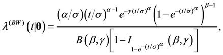
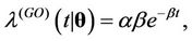
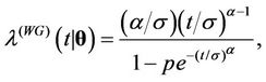
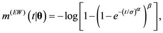
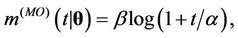
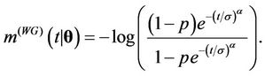
, . They are the Weibull (W), its generalisation, the exponentiated-Weibull (EW) (see for instance [33,34]) and their generalisation, the BetaWeibull (BW) [35-37] rate function. We also consider the Musa-Okumoto (MO) [38], the Goel-Okumoto (GO) [39] and a generalised form of Goel-Okumoto (GGO) rate functions as well as the Weibull-geometric (WG) rate function [40]. Those rate functions have the following form,


with , where
 is the incomplete Beta function with parameters
  and
and ,
,
 , and where
 ,
,  ,
,  ,
,  and
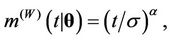
and . The associated mean functions are given, respectively, by


Remark. Note that in the case where ,
,  ,
,  , corresponds to the rate function given by
 . We also have that for
 , the rate function
  corresponds to
  and when
 , we have that
  is
is  (for more information see [36], where an analysis of the behaviour of
  in function of its parameters is presented). Observe that for
  the rate function
 ,
,  is decreasing as a function of
 . When
  we have that
  converges to the its equivalent Weibull rate function. We also have that for
  small,
  can be a decreasing, an increasing or an almost constant function of
  depending on the values of the parameters
  and
and  [40]. Note that if we take
  in
in , then we obtain
 .
.
The parameters of the models that must be estimated are ,
,  ,
, 
 and
and  when the Weibull, exponentiated-Weibull, Beta-Weibull, Musa-Okumoto, Goel-Okumoto, generalised Goel-Okumoto, and the Weibull-geometric models are used, respectively.
3. Bayesian Formulation of the Models
Take  a real number and assume that during the time interval
  there are
  days in which the concentration of a given pollutant surpasses a threshold of interest. Let
  indicate those days and let
  be the observed data.
The parameters of the models are estimated using a sample drawn from their respective posterior distributions. The posterior distribution of a parameter  given the data
 , indicated by
 , may be written as
 , where
  is the likelihood function of the model and
  is the prior distribution of
 . We are going to assume prior independence among the parameters. Since we have, by hypothesis, that a non-homogeneous Poisson model is assumed for the problem, then from [41,42], we have that
 (1)
(1)
where  and
and  are the rate and mean functions, respectively, of the Poisson process
 .
.
When the presence of change-points is allowed, then we have from [30,31,43,44], that the likelihood function takes the form,
 (2)
(2)
where , with
  the set of possible change-points, and where
  is the set of parameters of the respective model for
 , j = 2, 3,···, J, with
  and
and  the vectors of parameters in the case where
  and
and , respectively, and with
 , the respective rate function,
 .
.
Remark. The likelihood function in the case of the Weibull, exponentiated-Weibull, Musa-Okumoto, GoelOkumoto and generalised Goel-Okumoto rate functions may be found in [29,31,32,34]. Hence, in here we only present the expression for the likelihood function in the cases of the Beta-Weibull and Weibull-geometric rate functions.
Consider the Beta-Weibull rate function. In this case, we have that,
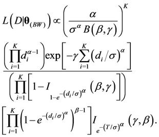 (3)
(3)
In the case of the Weibull-Geometric rate function, the likelihood function has the following form,
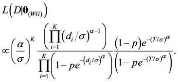 (4)
(4)
The prior distributions as well as their hyperparameters, which will be considered known, are presented in Section 4 when we apply the results to the ozone data from Mexico City.
Estimation of the parameters is going to be performed using a sample drawn form their respective complete marginal conditional posterior distribution using either the Gibbs sampling algorithm [45] internally implemented in the software WinBugs or a Gibbs sampling together with a Metropolis-Hastings algorithm [46,47] programmed in R (in the case of the model using the Beta-Weibull rate function). When using the software WinBugs, we only need to specify the likelihood function and the prior distributions. However, when using the programmes in R, we need to specify the complete marginal conditional distribution for each of the parameters involved in the models, which in the case of the BetaWeibull rate function (model with no change-point) are given by


Remark. Note the  function does not have an expression in terms of elementary functions. However, it can be estimated very precisely. [48] proposes an algorithm to do such estimate which is now implemented in R. That was used in this work.
Convergence of the algorithm is monitored using the analysis of the trace plots and in some cases the Gelman-Rubin test [49] is also used. In the case of the Beta-Weibull the Geweke test was considered (see [50]) in addition to visual inspection of the trace plots. Selection of the best model to fit the data set considered here is made by visual inspection of the plots of the accumulated observed and estimated means and also using the deviance information criterion (DIC) and the Bayes Discrimination Method (BDM). The deviance is defined by , where
  is the vector of parameters of the model,
  is the observed data,
  is the likelihood function of the model and
  is a constant that is not needed when comparing the models. The DIC [51] is given by
 , where
  is the deviance evaluated at the posterior mean
  and
and  is the effective number of parameters of the model. Smaller values of DIC indicate better models. In the case of the Bayes Discrimination Method, we have from [52] that the marginal likelihood function (MLF) of the whole data set
  for Model
 ,
,  is given by
 (5)
(5)
where  is the vector of parameters for Model
  and
and  is the joint prior distribution for
 . The Bayes Discrimination method prefers Model
  to Model
  if
if . Also, from [52] we have that
  may be approximated by the expression
  , where
  is the dimension of the vector of parameters
 ,
,  is the estimated posterior mode of
 ,
,  is the joint prior distribution of
  evaluated in
 ,
,  is minus the inverse Hessian matrix of
  evaluated at
 , and
, and  is the determinant of
 .
.
Remark. We have decided to use both the DIC and BDM as well as graphical methods to choose the model that best fits the data because in some cases the DIC selects the best model in accordance with the graphical fitting, but in some cases it does not. Hence, we have decided to use another discrimination methods in addition to the DIC. Therefore, using both methods we are able to compare their performance.
4. An Application to Mexico City Ozone Measurement
In this section we apply the models, presented in earlier sections, to the ozone measurements from the monitoring network of Mexico City. The Metropolitan Area of Mexico City is divided into five sections, namely, NE (Northeast), NW (Northwest), CE (Centre), SE (Southeast) and SW (Southwest) (see for instance [19,29] and www.sma.df.gob.mx). This division is the one that is currently used to declare environmental alerts in Mexico City. Hence, we are going to consider this splitting instead of taking another spatial approach.
Measurements are obtained minute by minute and the averaged hourly result is reported at each station. The daily maximum measurement for a given region is the maximum over all the maximum averaged values recorded hourly during a 24-hour period by each station placed in the region. The data used here correspond to the daily maximum ozone measurements taken from 01 January 2000 until 31 December 2008, giving a total of  observations. The mean concentration levels for regions NE, NW, CE, SE and SW are, respectively, 0.1026 ppm, 0.00923 ppm, 0.1087 ppm, 0.1085 ppm and 0.1246 ppm with respective standard deviation given by 0.0416, 0.0319, 0.0412, 0.0369 and 0.0456. We are going to analyse each region separately. Recall that the threshold considered here is 0.17 ppm. During the period of time
 , that threshold was surpassed in 197, 42, 202, 125 and 440 days in regions NE, NW, CE, SE, and SW, respectively.
The prior distributions as well as their hyperparameters are given as follows. We first consider the situation where no change-points are present. In the case of the Weibull rate function for all regions, the parameters  and
and  have uniform prior distributions defined on the intervals (0, 2) and (0, 100), respectively. When we consider the exponentiated-Weibull rate function we have the following. The parameter
  has a Gamma (a, b) prior distribution with hyperparamters
  and
and  for all regions. The parameter
  has a Gamma (1, c) prior distribution when considering regions NE, CE, SE and SW. In the case of regions NE, CE and SE the hyperparameter is
  and is
  for region SW. When we consider region NW,
  has a Gamma prior distribution with hyperparamters
  and
and . The parameter
  is such that for regions NE, CE, SE and SW its prior distribution is a uniform distribution defined on the interval (0, 100). In the case of region NW its prior distribution is a Gamma (
 ) distribution with hyperparameter
 . When taking into account the Beta-Weibull rate function for all regions and all parameters we consider Gamma prior distributions. The hyperparameters are, for all regions,
  in the case of the parameter
 ,
,  for the other parameters, and
  for the parameters
 ,
,  and
and  and
and  for the parameter
 . When the Musa-Okumoto rate function is considered,
  and
and  will have Gamma (500,000, 10) and Gamma (200,000, 10) prior distributions, respectively. When we consider the Goel-Okumoto rate function we have that
  and
and  have prior distributions Gamma (1200, 1) and Gamma (0.1, 1), respectively, for all regions. In the case of the generalised Goel-Okumoto we assume, for all regions, uniform prior distributions defined on the intervals (500, 2000) and (0.5, 1.5) for the parameters
  and
and , respectively. In the case of the parameter
 , a Gamma prior distribution with hyperparameters
  and
and  is considered for all regions. When we take into account the Weibull-geometric rate function two steps were considered. In the first step, for all regions, uniform prior distributions defined on the intervals (0, 2), (0, 100) and (0, 1) for the parameters
 ,
,  and
and , respectively, are considered. In the second step, based on the information provided by the first step, more informative prior distributions are taken. Hence, we have that for the parameters
  and
and  for all regions we use Gamma prior distributions as shown in Table 1.
In the case of the parameter  we take a Beta (
 ) prior distribution whose hyperparameters are
  for all regions and
 , for regions NE, CE, SE and SW, and is
  for region NW. (In here, Gamma (
 ) and Beta (
 ) are the Gamma and Beta distributions with means
  and
and  and variances
  and
and , respectively).
Remark. The prior distribution of the parameters as well as their hyperparameters were selected based on information provided by previous studies.
In all cases, a sample of size 3234, taken every 30th generated value after a burn-in period of 3000 steps was used to perform the estimation of the parameters. The DIC and MLF values used in the selection of the model that best fits the data are given in Table 2.
It is possible to see that the smallest value of the DIC is achieved, for all regions, when the Beta-Weibull rate function is considered. When considering the BDM, we have that the best model is the MO model for regions SE and CE, the BW model for region SW, and the WG with uniform prior distribution model for region NW. In the
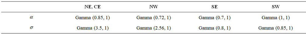
Table 1. Prior distribution for the parameters α and σ when the Weibull-geometric rate function is taken into account.

Table 2. DIC and marginal likelihood function (MLF) values for all regions and models without the presence of changepoints.
case of region NE, the selected model is the GGO model.
Besides the DIC and the BDM, a visual inspection of the fit of the observed and estimated accumulated means is also used. Hence, in Figure 1, we have the accumulated observed and estimated means when models W, EW, BW and WG with uniform prior distributions are considered. Plain solid line represents the accumulated observed mean and lines with ▲, ●, ■, and ♦, represent the estimated mean when using models W, EW, BW and WG, respectively.
Observing Figure 1 we may notice the following. The worst fit is given by the BW and EW rate functions in all regions with the exception of region NW. In that case, we have that the best fit is given by the BW rate function. Nevertheless, the worst fit still is provided by the EW rate function. The best fit in the other regions are given by either the Weibull or the Weibull-geometric rate function.
In Figure 2, we have the accumulated observed and estimated means when we consider the best model that fitted the data which is presented in Figure 1 (in this case we are taking the W rate function for regions NE, CE, SE and SW) and also models MO, GO and GGO. Again, plain solid line represents the accumulated observed mean and lines with ■, ♦, ● and ▲, represent the estimated means when the best fit from Figure 1, models MO, GGO and GO are considered, respectively.
We may observe from Figure 2 that for regions NE, CE, SE and SW the fit improves when using the GGO rate function instead of taking either the W or WG rate function. Nevertheless, in the case of region NW the fit is improved when using the MO rate function. Looking at the plots for region SW we also have that the MO model gives a very good approximation for the accumulated observed mean. In the case of regions NE, CE and SE, the fit provided by the MO model is not as good as the one given by the GGO model, but is still better than the fit provided by the other rate functions.
Remark. Even though the DIC and BDM criteria may select a given model, we may notice that it is worthwhile to use the graphical criterion as well.
In Table 3, we have the estimated posterior mean, standard deviation (indicated by SD) and the 95% credible intervals for all parameters and regions NE, CE, SE and SW, when the GGO model is used. We present the results only for that model because it is the one providing the best graphical fit for the regions considered. Note that region NW is not included since in that case the best fit is provided by the MO model followed by the BW rate function (The estimated value of the parameters of those rate functions are given in Table 4).
In Table 4, we give the estimated quantities of interest
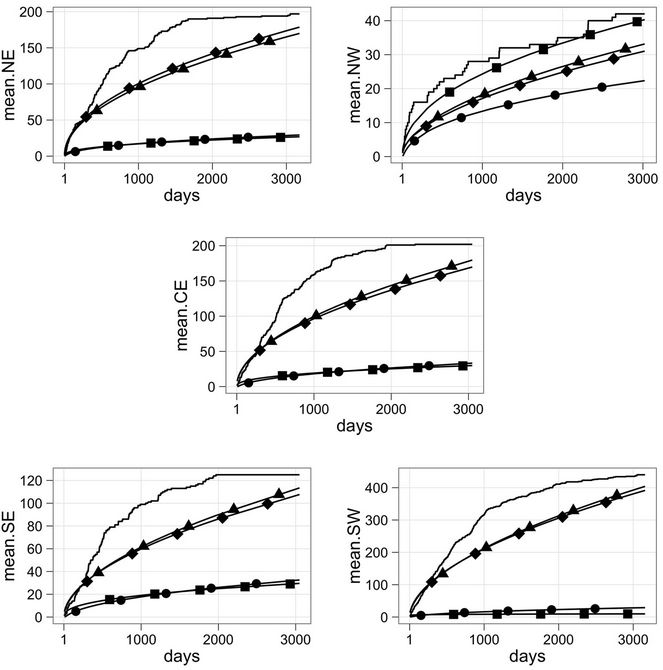
Figure 1. Accumulated observed and estimated means for all models and all regions. Solid plain line represents the accumulated observed mean. Lines with ■, ●, ▲, and ♦ correspond to the accumulated estimated mean when models Beta-Weibull, exponentiated-Weibull, Weibull and Weibull-geometric, respectively.
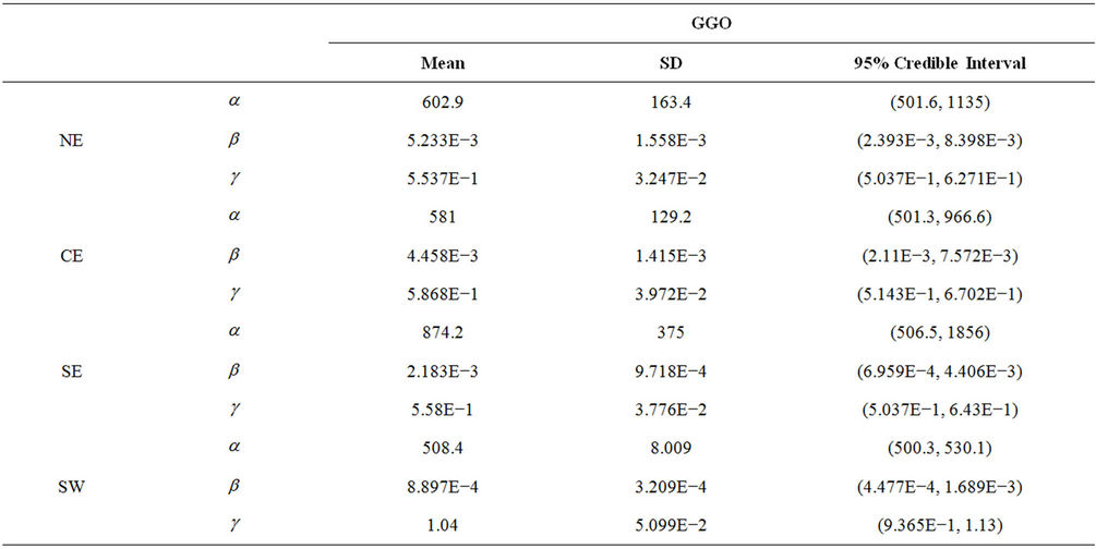
Table 3. Estimated mean, standard deviation (indicated by SD), and the 95% credible intervals for the parameters of the generalised Goel-Okumoto rate function without the presence of change-points and regions NE, CE, SE and SW.
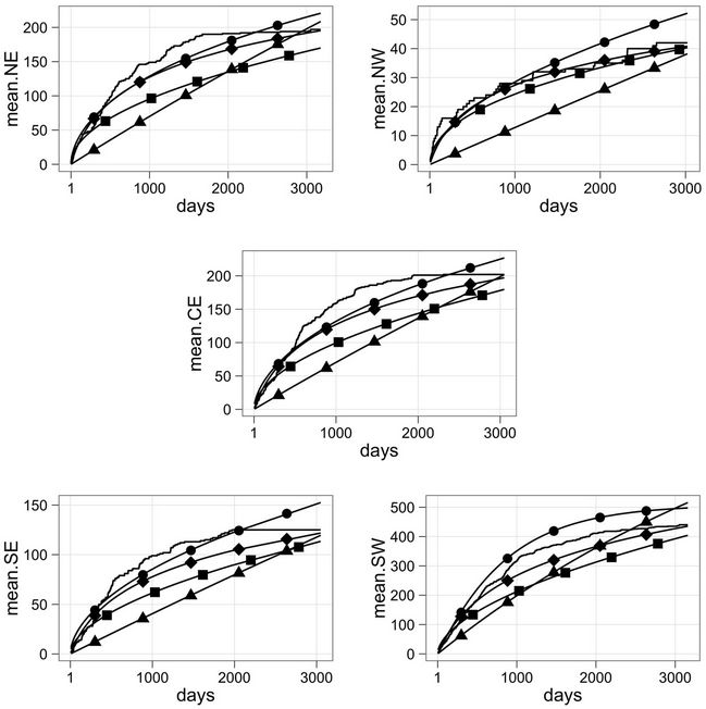
Figure 2. Accumulated observed and estimated means for all models and all regions. Solid plain line represents the accumulated observed mean. Lines with ■ correspond to the estimated Beta-Weibull accumulated function in the case of region NW and to the estimated Weibull accumulated mean in for the other regions, lines with ♦, ● and ▲, correspond to the accumulated estimated mean when the MO, GGO and GO rate functions are considered, respectively.

Table 4. Estimated mean, standard deviation (indicated by SD) and the 95% credible intervals for the parameters of the Musa-Okumoto and Beta-Weibull rate functions without the presence of change-points and regions NE, NW and SW.
when either the MO or the BW models are used and regions NE, NW and SW are considered. Note that besides region NW we also consider regions NE and SW. That is so because the MO model also gives a good fit for those regions in addition to the GGO model.
As can be seen from Figures 1 and 2, in some cases the model with presence of change-points should be considered as an option. Hence, for some of the models and regions we also allow the presence of one or two changepoints depending on the region and model. Following in that direction we consider the MO and GGO models with the presence of one change-point in the case of regions NE, CE, SE and SW. We also assume the presence of two change-points in the case of GGO model and data from region SE. The prior distributions taken in those cases are as follows. When the GGO model is considered, for all regions and cases (one and two change-points) we have that  and
and ,
,  , have uniform prior distributions defined on the intervals (500, 2000) and (0.1, 1), respectively. The parameter
  have a Gamma prior distribution with hyperparameters
  and
and . When one change-point is considered, we have that the change-point
  has an uniform prior distribution defined on the interval (0, 100) and in the case of two change-points, then
  and
and  have uniform prior distributions defined on the intervals (0, 500) and (1000, 1500), respectively. In the case of the MO model and one change-point, the change-point
  has the same prior distribution as in the case of the GGO model. The parameters
  and
and  have uniform prior distributions defined on the intervals (0, 500) and (1, 2500), respectively,
 .
.
Estimation of the parameters in the case of the GGO model with one-change point was performed using a sample of size 3234 obtained every 30th generated value after a burn-in period of 3000 iterations. When we consider the GGO model with two change-points, the inference was made using a sample of size 8333 taken every 30th generated value after a burn-in period of 150,000 steps.
Table 5 presents the value of the DIC and MLF for the regions and models where the presence of change-points is assumed.
Looking at Table 5 we have that, according to the deviance information criterion, for regions NE, CE and SW either the MO or the GGO with a change-point model could be chosen. However, when considering BDM we have that in all cases the GGO model with a change-point should be selected. In the case of region SE, when using the DIC, we have that either the MO with a change-point or the GGO model with two change-points could be selected. Nevertheless, when using the BDM we have that the MO model with a change-point is the one that should be selected.
When comparing the values given in Tables 2 and 5, we have that when using the DIC, for all regions, the selected model should be the Beta-Weibull model. When using the BDM we have that in the case of regions NE and CE the GGO model with a change-point should be used. However, when considering region SE, the MO model with a change-point is the one that should be selected. In the case of the remaining regions NW and SW, the selected result remains unchanged.
Figure 3 presents the plots of the estimated and observed accumulated means when models MO and GGO are considered and the presence of change-points is allowed (one change-point in the case of regions NE, CE, SE and SW and also two change-points in the case of region SE and model GGO). Plain solid lines represents the observed accumulated means and lines with ■ and ● represent the estimated accumulated means when the GGO and the MO models with one change-point are used, respectively. In the case of region SE, the line with ▲ represents the estimated accumulated mean when the GGO model with two change-points is considered.
Observing Figure 3, we may see that the GGO model with the presence of one change-point provides a very good fit in the case of regions NE and SW. Even though that model gives a good fit also in the case of region CE we have that the MO model with one change-point gives a better approximation. In the case of region SE both the MO model with one change-point and the GGO model with two change-points provide almost the same approximation and both are better than the one given by the GGO model with only one change-point.
Tables 6 and 7 present the estimated quantities of

Table 5. DIC and marginal likelihood function (MLF) values for the regions and models where the presence of change-points is allowed.
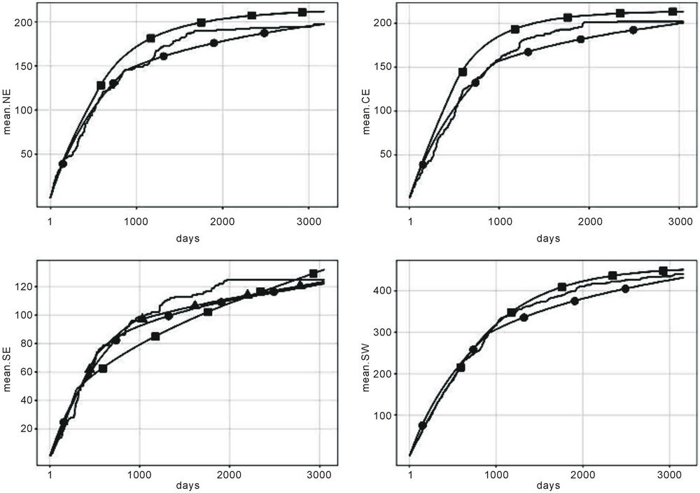
Figure 3. Accumulated observed and estimated means for all models with change-points and regions NE, CE, SE and SW. Solid plain line represents the accumulated observed mean. Lines with ■ correspond to the estimated GGO accumulated function with one change-point, those with ● correspond to the estimated MO accumulated function with one change-point and that with ▲, in the case of region SE, corresponds to the estimated GGO accumulated function with two change-points.
interest when we consider the GGO and the MO models with one change-point and regions NE, CE and SW and when we consider the GGO model with two change points and the MO model with one change-point and region SE.
Remark. The estimated parameters for all models considered here and for all regions can be found in https://sites.google.com/site/jmbarrios/recursos/result-reports-for-jep.
5. Discussion
In this paper we have considered several non-homogeneous Poisson models as possible models to explain the behaviour of the mean number of times that a given ozone threshold is surpassed in a time interval of interest by the daily maximum ozone concentration. The interest was to see which model fits better the ozone data from Mexico City obtained after a series of environmental measures were taken aiming to decrease the emission of pollutants, in particular, ozone precursors.
It is possible to see that depending on the criterion used, the selected model varied. That can be seen when looking at Tables 2 and 5, and Figures 1-3. Hence, when the deviance information criterion is used, the selected model, for all regions, was the one considering the BW rate function for the Poisson model. Contrasting this selection with the plots in Figures 1-3, we have that only in region NW that model provides a good graphical fit. That fit is only improved by the use of the MO rate function (see Figure 2). When using the Bayes discrimination method we may observe from Tables 2 and 5, that the model selected to best explain the ozone data varied according to region. Hence, we have that the GGO model with a change-point was the one selected when regions NE and CE were considered and the WG, MO with a change-point and BW models were the ones selected when we take into account regions NW, SE and SW, respectively. Note that the BW model was also the one selected for region SW when using the DIC, however,
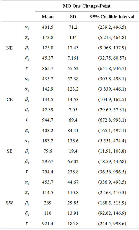
Table 6. Estimated mean, standard deviation and the 95% credible intervals for the parameters of the Musa-Okumoto rate function with the presence of one change-spoint for region NE, CE, SE and SW.
the fit of the estimated mean to the observed mean is not appropriate (see Figure 1). Based on the graphical fit we have that the GGO model with one change-point was the one providing the best approximation for region SW (see Figure 3). However, the MO model with a change-point also provides a good fit for the data from that region as well. Note that the model also gives a reasonable fit when considering the data from the last four years when considering regions CE and NE (see Figure 3) and also during the first two years of the measurements obtained in region NE. We may also notice that the MO model with one change-point provides a very good fit when taking into account the data from the first two years and regions NE and CE. The fit is not as good for the later years in the same regions. It is possible to see that for region SE either the MO model with one change-point or the GGO model with two change-points provides a reasonable fit for the first six years, however, the fit becomes worse in the final years of the observational period.
Remark. Note that the change-point for regions NE, CE and SW corresponds to a day in May, in June and in May 2001, respectively. In the same manner those for region SE correspond to a day in May in 2001 and another in July 2002. Hence, we may see that changepoints start to occur as soon as the environmental measures taken until the year 2000 start to have an effect on the ozone concentration levels.
Even thought the BW rate function is a more complex function when compared to the others considered here, we have that the BW programmed in R was about six times faster than when using, the particular case of BW, the EW rate function and the WinBugs software. One drawback though, is that we had a poor mixing when considering sampling from the posterior distribution of the variable  That shortcoming was corrected by considering more iterations of the Metropolis-Hastings step for that variable before moving on to the next step in the Gibbs sampling part of the algorithm. In that case, we run ten steps of the Metropolis-Hastings algorithm for the variable
  against one step for each of the remaining parameters of the BW rate function.
When comparing the graphical fit with the results from previous works we have the following. If we consider the analysis performed by [29] using the EW and W models and data from 01 January 1998 to 31 December 2004, we have that for all regions the selected model using the Bayes information and the deviance information criteria was the one considering the particular case of Weibull rate function. In terms of graphical adjustment we have that the Weibull rate function gives a much better fit when considering the 1998-2004 data for all regions. In [30], we have the use of the W, MO, GO and GGO rate functions applied to the overall maximum ozone measurements from 01 January 1998 to 31 December 2004. Even though the time interval in which the data was collected was the same as in [29], we have that the regional division of the Metropolitan Area was not taken into account. The model selection was performed using the deviance information criterion and the model chosen was the GGO. This model was also selected for regions NE and CE when using the Bayes discrimination method and the 2000-2008 data. However, when using the DIC, in all regions, the selected model was the BW. When observing Figure 2 and when comparing to the adjustment given by the GGO model when the data 1998-2004 is used, we have an almost perfect fit in the latter. If we compare the values of the parameters estimated, we have that the value of the  when using the 1998-2004 data is almost the double of the value obtained when using the
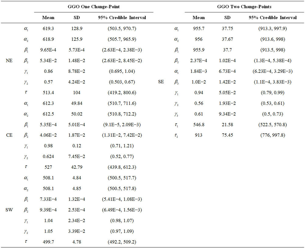
Table 7. Estimated mean, standard deviation (indicated by SD), and the 95% credible intervals for the parameters of the generalised Goel-Okumoto rate function with the presence of either one or two change-points for regions NE, CE, SE and SW.
2000-2008 data for all regions with the exception of region SE. In the case of the other parameters, the ones estimated using the data 2000-2008 for region SW are the ones that have more similarity with the ones estimated using the 1998-2004 data (see [30]). That can be explained by the fact that region SW is, in almost all cases, the one that contributes to most of the days in which the threshold 0.17 ppm is surpassed and hence, in a way dictates the behaviour of the overall measurements.
The W, MO and GGO model were also used in [32]. In there, the regional division of the Metropolitan Area was taken into account, but the data set was composed by the daily maximum measurements obtained from 01 January 2003 to 31 December 2009. The selection of the model that best fit the data from each region was performed using the Bayes discrimination method and visual inspection of the graphical adjustment between the estimated and observed accumulated means. According to the Bayes discrimination criterion the best model to explain the behaviour of the data was the Weibull rate function (either with  having an uniform prior distribution or having a Beta). This presents a very different result as the one when using the 2000-2008 data (see Tables 2 and 5). In terms of graphical adjustment we have that the behaviour of the data 2003-2009 is also different from the 2000-2008 data. In the former data set we have that the W model fits better the data from region NE, the GGO is the one chosen for region NW, and in the case of regions CE and SE, even though the GGO model fits adequately, we have that towards the end of the observational period the MO model could also be a choice. In the case of region SW we have that any of the models provides a very good graphical adjustment. This behaviour is not repeated in the 2000-2008 data. We may observe from Figure 1 that the Weibull model does not provide a good adjustment. In both sets of data the MO model may also be used as an alternative to the GGO model, but in the case of the 2003-2009 data the fit of the MO function, when it occurs, is mainly in later years. In the case of the 2000-2008 data, the MO and GGO models needed the inclusion of change-points so the fit could be a good one.
Remark. The selection of the prior distributions and their hyperparameters in the BW model was made using information obtained when the EW and W models were considered. Even though, convergence of the MCMC algorithm was achieved in the BW model with the prior distributions considered here, several prior distributions were tested. The common factors in all tested distributions were that they had the same mean and belonged to the same parametric family. The only difference was that they had different variances. As a result of the tests, we have observed that as the variance increased the time needed to achieve convergence of the MCMC sampler also increased and in some cases it was not achieved at all during the time the algorithm was left to run. As an example, in the case of the region NW region we needed an additional 100,000 steps to have that the MCMC algorithm converged and in the case of regions NE, CE, SE, SW an additional 200,000 iterations were necessary. When we considered smaller variance we have obtained either a no satisfactory or a null acceptance rate for the Metropolis-Hastings part of the algorithm.
Some of the rate functions considered here for the Poisson process are commonly used in reliability theory. Their use in the present work is justified because of the very nature of the problem studied here. Additionally, depending on the value of the parameters present in their formulation, we may account for the many different behaviours that might be present in the data set considered.
Other threshold values could also be used. When considering values smaller than 0.17 ppm we may lose the Poisson property and hence some types of dependence may be considered. As an example of that we have [53] where the threshold 0.11 ppm is used and [54] where the value 0.14 ppm is considered.
6. Acknowledgements
We thank an anonymous reviewer for the comments sent that helped clarify some points in the text. This work was financially supported by the project PAPIIT number IN104110-3 of the Dirección General de Apoyo al Personal Académico of the Universidad Nacional Autónoma de México, Mexico, and is part of JMB’s Ph.D. Thesis. JMB was partially funded by the Consejo Nacional de Ciencias y Tecnologia, Mexico, through the Ph.D. Scholarship number 210347. JAA was partially funded by the Conselho Nacional de Pesquisa, Brazil, grant number 300235/2005-4.
REFERENCES
- M. L. Bell, A. McDermontt, S. L. Zeger, J. M. Samet and F. Dominici, “Ozone and Short-Term Mortality in 95 US Urban Communities, 1987-2000,” Journal of the American Medical Society, Vol. 292, 2004, pp. 2372-2378.
- M. L. Bell, R. Peng and F. Dominici, “The ExposureResponse Curve for Ozone and Risk of Mortality and the Adequacy of Current Ozone Regulations,” Environmental Health Perspectives, Vol. 114, 2005, pp. 532-536. doi:10.1289/ehp.8816
- M. L. Bell, R. Goldberg, C. Rogrefe, P. L. Kinney, K. Knowlton, B. Lynn, J. Rosenthal, C. Rosenzwei and J. A. Patz, “Climate Change, Ambient Ozone, and Health in 50 US Cities,” Climate Change, Vol. 82, No. 1-2, 2007, pp. 61-76. doi:10.1007/s10584-006-9166-7
- W. J. Gauderman, E. Avol, F. Gililand, H. Vora, D. Thomas, K. Berhane, R. McConnel, N. Kuenzli, F. Lurmman, E. Rappaport, H. Margolis, D. Bates and J. Peter, “The Effects of Air Pollution on Lung Development from 10 to 18 Years of Age,” New England Journal of Medicine, Vol. 351, 2004, pp. 1057-1067. doi:10.1056/NEJMoa040610
- G. Likens (Lead Author), W. Davis, L. Zaikowski and S. C. Nodvin (Topic Editors), “Acid Rain, 2011,” In: J. Cutler, ed., Encyclopedia of Earth, Environmental Information Coalition, National Council for Science and the Environment, Cleveland, 2011. http://www.eoearth.org/article/Acid_rain
- D. Loomis, V. H. Borja-Arbuto, S. I. Bangdiwala and C. M. Shy, “Ozone Exposure and Daily Mortality in Mexico City: A Time Series Analysis,” Health Effects Institute Research Report, Vol. 75, 1996, pp. 1-46.
- M. R. O’Neill, D. Loomis and V. H. Borja-Aburto, “Ozone, Area Social Conditions and Mortality in Mexico City,” Environmental Research, Vol. 94, No. 3, 2004, pp. 234-242. doi:10.1016/j.envres.2003.07.002
- WHO (World Health Organization), “Air Quality Guidelines—2005. Particulate Matter, Ozone, Nitrogen Dioxide and Sulfur Dioxide,” World Health Organization Regional Office for Europe, 2006.
- NOM, “Modificación a la Norma Oficial Mexicana NOM-020-SSA1-1993 (In Spanish),” Diario Oficial de la Federación, 2002.
- J. Horowitz, “Extreme Values from a Nonstationary Stochastic Process: An Application to Air Quality Analysis,” Technometrics, Vol. 22, No. 4, 1980, pp. 469-482. doi:10.1080/00401706.1980.10486195
- E. M. Roberts, “Review of Statistics Extreme Values with Applications to Air Quality Data. Part I. Review,” Journal of the Air Pollution Control Association, Vol. 29, No. 7, 1979, pp. 632-637. doi:10.1080/00022470.1979.10470856
- E. M. Roberts, “Review of Statistics Extreme Values with Applications to Air Quality Data. Part II. Applications,” Journal of the Air Pollution Control Association, Vol. 29, No. 6, 1979, pp. 733-740. doi:10.1080/00022470.1979.10470835
- R. L. Smith, “Extreme Value Analysis of Environmental Time Series: An Application to Trend Detection in Ground-Level Ozone,” Statistical Sciences, Vol. 4, No. 4, 1989, pp. 367-393. doi:10.1214/ss/1177012400
- J. B. Flaum, S. T. Rao and I. G. Zurbenko, “Moderating Influence of Meteorological Conditions on Ambient Ozone Concentrations,” Journal of the Air & Waste Management Association, Vol. 46, No. 1, 1996, pp. 33-46. doi:10.1080/10473289.1996.10467439
- N. Gouveia and T. Fletcher, “Time Series Analysis of Air Pollution and Mortality: Effects by Cause, Age and Socio-Economics Status,” Journal of Epidemiology and Community Health, Vol. 54, No. 10, 2000, pp. 750-755. doi:10.1136/jech.54.10.750
- U. Kumar, A. Prakash and V. K. Jain, “A Multivariate Time Series Approach to Study the Interdependence among O3, NOx and VOCs in Ambient Urban Atmosphere,” Environmental Modeling & Assessment, Vol. 14, No. 5, 2010, pp. 631-643. doi:10.1007/s10666-008-9167-1
- M. Lanfredi and M. Macchiato, “Searching for Low Dimensionality in Air Pollution Time Series,” Europhysics Letters, Vol. 40, No. 6, 1997, pp. 589-594. doi:10.1209/epl/i1997-00504-y
- J.-N. Pan and S.-T. Chen, “Monitoring Long-Memory Air Quality Data Using ARFIMA Model,” Environmetrics, Vol. 19, No. 2, 2008, pp. 209-219. doi:10.1002/env.882
- L. J. Álvarez, A. A. Fernández-Bremauntz, E. R. Rodrigues and G. Tzintzun, “Maximum a Posteriori Estimation of the Daily Ozone Peaks in Mexico City,” Journal of Agricultural, Biological Statistics, Vol. 10, No. 3, 2005, pp. 276-290. doi:10.1198/108571105X59017
- J. Austin and H. Tran, “A Characterization of the Weekday-Weekend Behavior of Ambient Ozone Concentrations in California,” In: Air Pollution VII, WIT Press, Southampton, 1999, pp. 645-661.
- J. A. Achcar, H. C. Zozolotto and E. R. Rodrigues, “Bivariate Volatility Models Applied to Air Pollution Data,” Revista Brasileira de Biologia, Vol. 26, 2008, pp. 67-81.
- J. A. Achcar, H. C. Zozolotto and E. R. Rodrigues, “Bivariate Stochastic Volatility Models Applied to Mexico City Ozone Pollution Data,” In: G. C. Romano and A. G. Conti, Eds., Air Quality in the 21st Century, Nova Publishers, New York, 2010, pp. 241-267.
- J. A. Achcar, E. R. Rodrigues and G. Tzintzun, “Using Stochastic Volatility Models to Analyse Weekly Ozone Averages in Mexico City,” Environmental and Ecological Statistics, Vol. 18, No. 2, 2011, pp. 271-290. doi:10.1007/s10651-010-0132-1
- G. Huerta and B. Sansó, “Time-Varying Models for Extreme Values,” Environmental and Ecological Statistics, Vol. 14, No. 3, 2007, pp. 285-299. doi:10.1007/s10651-007-0014-3
- L. W. Davis, “The Effect of Driving Restrictions on Air Quality in Mexico City,” Journal of Political Economy, Vol. 116, No. 1, 2008, pp. 39-81. doi:10.1086/529398
- M. Zavala, S. C. Herndon, E. C. Wood, T. B. Onasch, W. B. Knighton, L. C. Marr, C. E. Kolb and L. T. Molina, “Evaluation of Mobile Emissions Contributions to Mexico City’s Emissions Inventory Using on Road and Cross-Road Emission Measurements and Ambient Data,” Atmospheric Chemistry and Physics, Vol. 9, No. 17, 2009, pp. 6305-6317. doi:10.5194/acp-9-6305-2009
- J. S. Javits, “Statistical Interdependencies in the Ozone National Ambient Air Quality Standard,” Journal of the Air Pollution Control Association, Vol. 30, No. 1, 1980, pp. 58-59. doi:10.1080/00022470.1980.10465918
- A. E. Raftery, “Extreme Value Analysis of Environmental Time Series: An Application to Trend Detection in Ground-Level Ozone,” Statistical Sciences, Vol. 4, No. 4, 1989, pp. 378-381. doi:10.1214/ss/1177012401
- J. A. Achcar, A. A. Fernández-Bremauntz, E. R. Rodrigues and G. Tzintzun, “Estimating the Number of Ozone Peaks in Mexico City Using a Non-Homogeneous Poisson Model,” Environmetrics, Vol. 19, No. 5, 2008, pp. 469-485. doi:10.1002/env.890
- J. A. Achcar, E. R. Rodrigues, C. D. Paulino and P. Soares, “Non-Homogeneous Poisson Processes with a Change-Point: An Application to Ozone Exceedances in Mexico City,” Environmental and Ecological Statistics, Vol. 17, No. 4, 2010, pp. 521-541. doi:10.1007/s10651-009-0114-3
- J. A. Achcar, E. R. Rodrigues and G. Tzintzun, “Using Non-Homogeneous Poisson Models with Multiple ChangePoints to Estimate the Number of Ozone Exceedances in Mexico City,” Environmetrics, Vol. 22, No. 1, 2011, pp. 1-12. doi:10.1002/env.1029
- E. R. Rodrigues, J. A. Achcar and J. Jara-Ettinger, “A Gibbs Sampling Algorithm to Estimate the Occurrence of Ozone Exceedances in Mexico City,” In: D. Popovic, Ed., Air Quality: Models and Applications, InTech Open Access Publishers, 2011, pp. 131-150.
- G. S. Muldholkar, D. K. Srivastava and H. Friemer, “The Exponentiated-Weibull Family: A Reanalysis of the BusMotor Failure Data,” Technometrics, Vol. 37, No. 4, 1995, pp. 436-445. doi:10.1080/00401706.1995.10484376
- J. E. Ramrez-Cid and J. A. Achcar, “Bayesian Inference for Nonhomogeneous Poisson Processes in Software Reliability Models Assuming Nonmonotonic Intensity Functions,” Computational Statistics and Data Analysis, Vol. 32, No. 2, 1999, pp. 147-159. doi:10.1016/S0167-9473(99)00028-6
- F. Famoye, C. Lee and O. Olumolade, “The Beta-Weibull Distribution,” Journal of Statistical Theory and Practice, Vol. 4, 2005, pp. 121-136.
- C. Lee, F. Famoye and O. Olumolade, “The Beta-Weibull Distributions: Some Properties and Applications to Censored Data,” Journal of Modern Applied Statistical Methods, Vol. 6, 2007, pp. 173-186.
- G. M. Cordeiro, et al., “Closed form Expressions for the Moments of the Beta-Weibull Distribution,” Annals of the Brazilian Academy of Sciences, Vol. 83, 2011, pp. 357- 373.
- J. D. Musa and K. Okumoto, “A Logarithmic Poisson Execution Time Model for Software Reliability Measurement,” Proceedings of Seventh International Conference on Software Engineering, Orlando, 1984, pp. 230- 238.
- A. L. Goel and K. Okumoto, “An Analysis of Recurrent Software Failures on a Real-Time Control System,” Proceedings of ACM Conference, Washington DC, 1978, pp. 496-500.
- W. Barreto-Souza, A. L. de Morais and G. M. Cordeiro, “The Weibull-Geometric Distribution,” Journal of Statistical Computation and Simulation, Vol. 81, No. 5, 2011, pp. 645-657. doi:10.1080/00949650903436554
- D. R. Cox and P. A. Lewis, “Statistical Analysis of Series Events,” Chapman and Hall, Methuen, 1966.
- J. F. Lawless, “Statistical Models and Methods for Lifetime Data,” John Wiley and Sons, New York, 1982.
- J. A. Achcar, E. Z. Martnez, A. Rufino-Neto , C. D. Paulino and P. Soares, “A Statistical Model Investigating the Prevalence of Tuberculosis in New York Using Counting Processes with Two Change-Points,” Epidemiology and Infection, Vol. 136, No. 12, 2008, pp. 1599-1605. doi:10.1017/S0950268808000526
- T. E. Yang and L. Kuo, “Bayesian Binary Segmentation Procedure for a Poisson Process with Multiple ChangePoints,” Journal of Computational and Graphical Statistics, Vol. 10, No. 4, 2001, pp. 772-785. doi:10.1198/106186001317243449
- A. E. Gelfand and A. F. M. Smith, “Sampling-Based Approaches to Calculating Marginal Densities,” Journal of the American Statistical Association, Vol. 85, No. 410, 1990, pp. 398-409. doi:10.1080/01621459.1990.10476213
- N. Metropolis, A. Rosenbluth, M. Rosenbluth, A. Teller and E. Teller, “Equations of State Calculations by fast Computing Machine,” Journal of Chemical Physics, Vol. 21, No. 6, 1953, pp. 1087-1091. doi:10.1063/1.1699114
- W. K. Hastings, “Monte Carlo Sampling Methods Using Markov Chains and Their Applications,” Biometrika, Vol. 57, No. 1, 1970, pp. 97-109. doi:10.1093/biomet/57.1.97
- A. R. Didonato and A. H. Morris, “Algorithm 708: Significant Digit Computation of the Incomplete Beta Function Ratios,” Transactions on Mathematical Software, Vol. 18, No. 3, 1992, pp. 360-373. doi:10.1145/131766.131776
- A. Gelman and D. B. Rubin, “Inference from Iterative Simulation Using Multiple Sequences,” Statistical Sciences, Vol. 7, No. 4, 1992, pp. 457-511. doi:10.1214/ss/1177011136
- J. Geweke, “Evaluating the Accuracy of Sampling-Based Approaches to the Calculation of Posterior Moments,” In: J. M. Bernardo, J. O. Berger, A. P. Dawid and A. F. M. Smith, Eds., Bayesian Statistics, Vol. 4, Clarendon Press, Oxford, 1992, pp. 169-193.
- D. J. Spiegelhalter, N. G. Best, B. P. Carlin and A. van der Linde, “Bayesian Measures of Model Complexity and Fit,” Journal of the Royal Statistical Society Series B, Vol. 64, No. 4, 2002, pp. 583-639. doi:10.1111/1467-9868.00353
- A. E. Raftery, “Hypothesis Testing and Model Selection,” In: W. Gilks, S. Richardson and D. J. Speigelhalter, Eds., Markov Chain Monte Carlo in Practice, Chapman and Hall, London, 1996, pp. 163-187.
- J. A. Achcar, E. R. Rodrigues and M. H. Tarumoto, “Using Counting Processes to Estimate the Number of Ozone Exceedances: An Application to the Mexico City Measurements,” Proceedings of the 58th ISI World Statistics Congress, Dublin, 21-16 August 2011. http://isi2011.congressplanner.eu/25
- J. A. Achcar, E. Cepeda-Cuervo and E. R. Rodrigues, “Weibull and Generalised Exponential Overdispersion Models with an Application to Ozone Air Pollution,” Journal of Applied Statistics, Vol. 39, No. 9, 2012, pp. 1953-1963. doi:10.1080/02664763.2012.697132
NOTES
*Corresponding author.